What are Mathematical Functions?

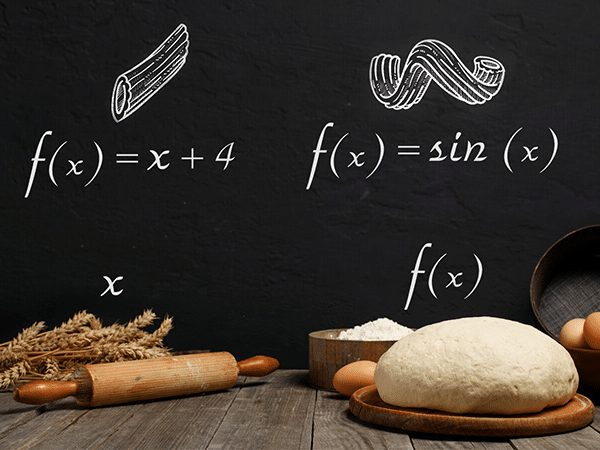
The topic of today’s post is mathematical functions. Functions are such a fundamental part of mathematics that you’re certain to encounter them almost everywhere.

Recently, I started a small series on numbers and arithmetic, in order to begin exploring the intuition of basic mathematical concepts that most of us take for granted. And these concepts themselves are the building blocks of more advanced concepts, including more advanced concepts in probability theory.

But to fully understand them, we also need to know the details and intuition of some general mathematical tools which we’re going to rely on along the way. Well, functions are first in line!

As a concept, mathematical functions are nothing complicated. However, they’re not necessarily always explained in the most intuitive way and this usually gives a wrong impression. Let’s start with the word “function” itself. What’s the first thing you associate it with? How would you define it?

I personally think of the word function as a sort of action. Something that does something (typically) useful. For example, a refrigerator has the function of cooling things down. A clock has the function of keeping track of time, as well as the function of displaying the current time at any given moment. Trains have the function of transporting things from point A to point B. A nose has the function of detecting and differentiating odors. You get the idea.

The word itself comes from the Latin functio which roughly translates to something like “a performance” or “an execution”.

This is the general concept but it’s a bit informal, isn’t it? Well, functions also exist in the world of mathematics. And, as you know, mathematics doesn’t really like informality too much. Hence, the mathematical definition of the concept is much more specific and rigorous. As you’ll see, however, this definition isn’t too far from the one we use in everyday language.

Functions in mathematics

The concept of a function in mathematics existed only implicitly until the 17th century. The people who first formally introduced it (and the term itself) were the legendary mathematicians Gottfried Leibniz and Johann Bernoulli.

Leibniz was a German mathematician who, together with Isaac Newton, laid the foundations for modern calculus. Bernoulli, on the other hand, was a Swiss mathematician and another brilliant member of the Bernoulli family. Namely, he was the younger brother of Jacob Bernoulli whom you might remember from my post about the Bernoulli distribution.

Speaking of which, if you’ve been following my posts related to probability distributions, you’ve already encountered functions. In my introductory post I informally defined a function as something that takes some value, does some calculation with it, and returns another value.

I specifically talked about the probability mass function (PMF) of a discrete probability distribution and the probability density function (PDF) of a continuous probability distribution. Their role is to associate elements of the sample space of a random variable with their respective probabilities or probability densities.

So, in mathematics functions are also things that do something. In the case of PMFs and PDFs, that something is associating outcomes with their probabilities. But what can we say about mathematical functions in general?

Well, think of them as an input-output machine. A function is something that accepts a certain set of input values and, based on each value, returns a specific output value. In the case of PMFs, for example, the input values are the possible outcomes of a random variable and the output values are their respective probabilities.

Now let’s dig a little deeper and look at a more formal definition.

Functions as associations between sets

Between the 17th and the 19th centuries, functions still had a rather informal definition. But in the 19th century a general effort to formalize mathematics had begun and it was during that period that set theory emerged as the foundation for mathematics as a whole.

In set theoretic terms, you can think of a function as a rule that associates each element from one set to exactly one element from another set. Not clear yet? Let’s break this down.

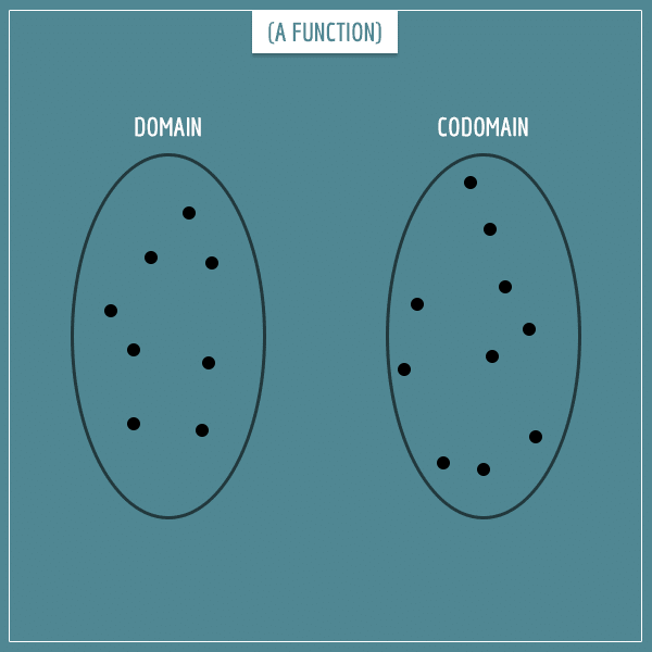
First, we need a set on which to define the function. That is, the set whose elements the function takes as input. This is called the domain of the function.

Second, we need another set with which the elements of the domain should be associated. That is, a set whose elements are the possible outputs of the function. This is called the codomain.

The image below represents the two sets and the black circles inside them are the elements of those sets:

Finally, we need to specify some rule that associates each element in the domain to exactly one element in the codomain:

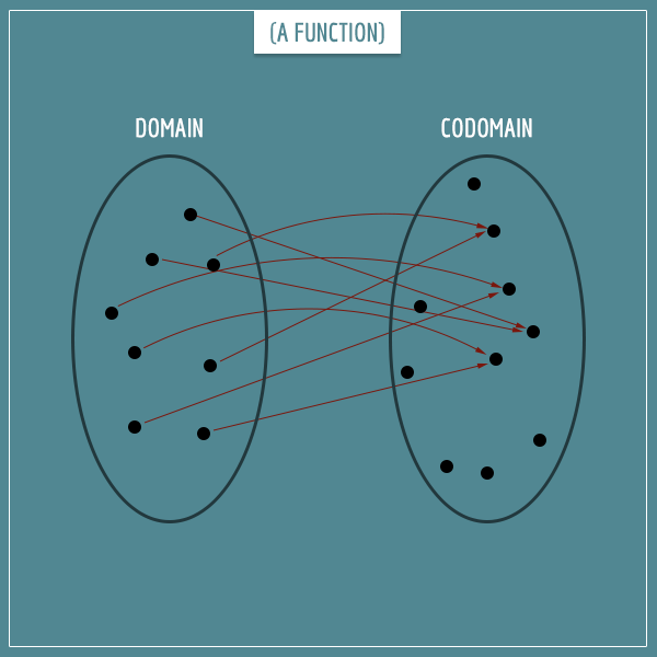
Notice that all elements in the domain have arrows pointing to one element in the codomain. But only 4 of the elements in the codomain are reached by those arrows:

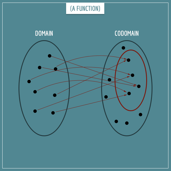
This subset of the codomain (the red ellipse) is called the range of the function and represents the set of its actual outputs.

Notation

In mathematics, the most common convention for expressing functions looks like this:

   

Functions are typically given temporary names in a certain context and one of the most common names is simply the letter ‘f’. The input is represented by a variable written in parentheses right after the function and is often called ‘x’. And the output variable is given after the equals sign and is typically labeled ‘y’.

You can read this as “f of x is equal to y”.

Well, this is pretty much the big picture. Now let’s look at some examples to get a better intuitive feeling for all these concepts.

Examples

Mapping countries to languages

Let’s say we have the set of all currently existing countries in the world. Let’s call this set “Countries”:

Countries = {Argentina, France, Nigeria, India, …}

And let’s say we have another set called “Languages” which contains all world languages (both currently existing, as well as dead languages):

Languages = {English, Dutch, Latin, Turkish, Spanish, Malagasy, …}

And now let’s define a function called “CountryLanguage”. This function expects a country name as input and returns the most commonly spoken language in that country as output. Here’s a few examples:

• CountryLanguage(USA) = English
• CountryLanguage(Argentina) = Spanish
• CountryLanguage(Madagascar) = Malagasy
• CountryLanguage(Bulgaria) = Bulgarian

In this example, the Countries set is the domain and the Languages set is the codomain of the CountryLanguage function. And the range is the subset of Languages that are actually most common in at least one currently existing country. That is, dead languages like Latin and minority languages like Romani aren’t part of the range, even though they are in the codomain.

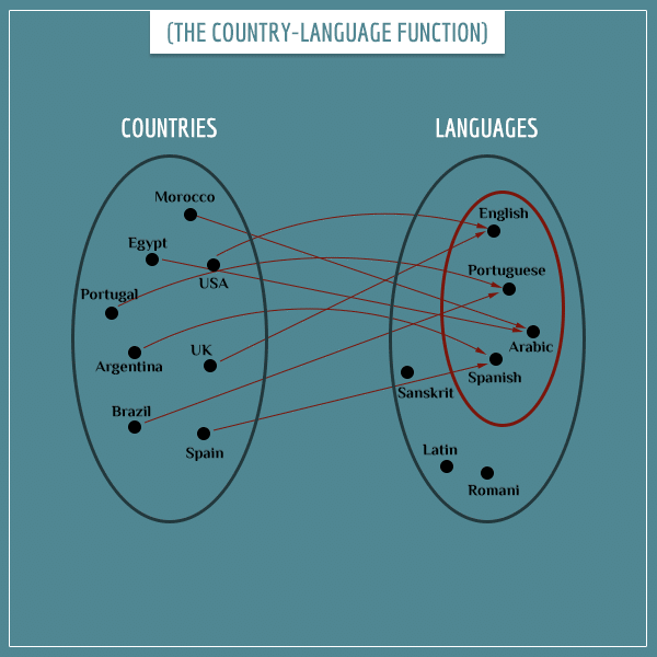
By analogy to reading f(x) = y as “f of x is equal to y”, you can read an expression like CountryLanguage(Argentina) = Spanish as “CountryLanguage of Argentina is equal to Spanish”.

Mapping French words to English words

Another example of a function is an actual dictionary, like a French-English dictionary. In this case we can simply call the function “Meaning” with examples like:

• Meaning(bonjour) = hello
• Meaning(enfant) = child
• Meaning(fleur) = flower

In this example, the set of all French words is the domain and the set of all English words is the codomain. And the range is the subset of English words that have a corresponding meaning in French (because that’s not always the case). Now, there are also French words with no direct translation to English. So, to be pedantic, we need to constrain the domain of the Meaning function to only those French words with a direct translation. That’s because a function is required to be defined for all elements in its domain.

In the examples so far, we’ve been dealing with finite sets, both for the domain and the codomain. But you can also define functions on infinite sets. In fact, the domains of most interesting mathematical functions are infinite.

Mapping (infinite) sets of numbers

In my overview post on discrete probability distributions, I discussed finite versus infinite sample spaces where the difference is that the former are finite sets, whereas the latter are infinite. There we were mostly concerned with the infinite set of natural numbers but I also mentioned other infinite sets, like the rational numbers and the real numbers (source for the images below):

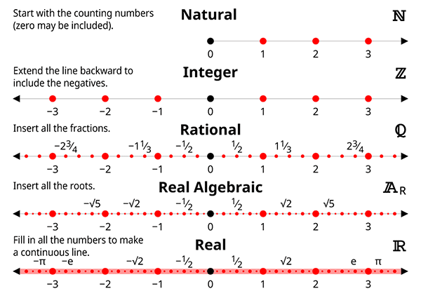
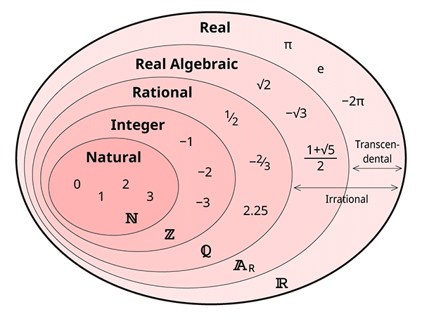
If you need more intuition about these numbers sets, check out my dedicated series I mentioned in the beginning.

Anyway, functions defined on infinite sets follow the same principles. The main difference is that here you can’t simply list all associations, since they’re infinite. Instead, you need an explicit rule that defines what output should be returned based on any input in the domain. Here’s an example:

   

We can define this function on the full set of real numbers. Hence, this function takes any real number and returns that number multiplied by 2. A few concrete examples are: , , , and so on.

If we define the codomain of the function to also be the set of real numbers, we finally see an example of a function where the range is the same as the codomain. And notice that there’s nothing wrong with having the same set as both the domain and the codomain.

You can also define functions on finite and infinite subsets of the real numbers. In fact, PMFs are a perfect example of functions whose domain is the set of natural numbers or any of its subsets. Their codomain is the set of real numbers and their range is the interval [0, 1], since probabilities are real numbers between 0 and 1.

The graph of a function

A function is a special kind of relation between two sets — the domain and the codomain. Namely, one that relates each element in the domain to exactly one element in the codomain. But you can view the function itself as a set as well. In particular, you can view it as a set of ordered pairs where the first element in a pair (x) is a possible input and the second element (y) is the corresponding output. The notation for an ordered pair is (x, y).

For example, take the function called LetterType. Its domain is the set of letters in the Latin alphabet and its codomain is the set {0, 1, 2}. It takes a letter from the alphabet and returns 1 if its a vowel, 0 if its a consonant, and 2 if it can be both. For example, LetterType(A) = 1, LetterType(B) = 0, LetterType(W) = 2, and so on.

We can represent this as a set containing the following ordered pairs:

{(A, 1), (B, 0), (C, 0), (D, 0), (E, 1), (F, 0), (G, 0), (H, 0), (I, 1), (J, 0), (K, 0), (L, 0), (M, 0), (N, 0), (O, 1), (P, 0), (Q, 0), (R, 0), (S, 0), (T, 0), (U, 1), (V, 0), (W, 2), (X, 0), (Y, 2), (Z, 0)}

Functions defined on infinite domains can also be represented as graphs, but obviously we can’t write the full set. Still, we can list at least some elements of the graph. For example, here’s a few elements from the set of the function from the previous section:

{(0, 0), (1, 2), (-3, -6), (2.5, 5), (π, 2π), (-7.5, -15), …}

Among other things, graphs allow us to visualize functions by plotting them. Which is especially useful for functions with infinite domains.

Plotting functions on a Cartesian coordinate system

I’ve implicitly assumed knowledge about Cartesian coordinate systems in most of my posts. But now is a good time to officially introduce them.

They were invented around the same time as functions by René Descartes, another great mathematician and philosopher. A Cartesian coordinate system consists of two perpendicular axes, each representing the real number line (the last line from the image in the previous section):

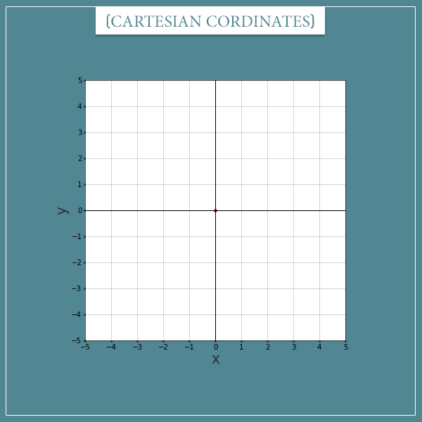
The two perpendicular axes form an infinite two-dimensional plane. Well, here I’m only showing the part of the plane spanned by the segments [-5, 5] of the axes.

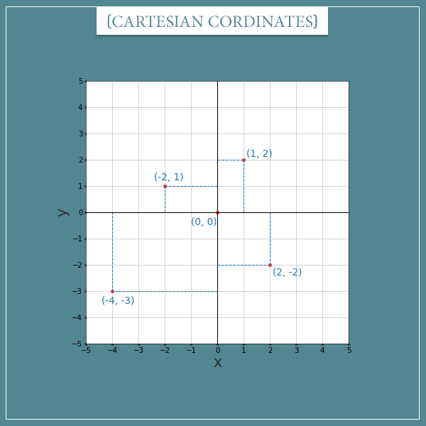
This coordinate system allows us to plot pairs of numbers as points on the plane. You already see one of them — the point with coordinates (0, 0). This is commonly called the origin of the coordinate system.

Plotting other points is easy enough. You can basically draw imaginary dashed lines from the corresponding points on the two axes and plot the point where they intersect. For example, let’s also plot the points (1, 2), (-2, 1), (-4, -3), and (2, -2) (along with the origin (0, 0)):

Plotting functions from their graphs

What’s cool about this is that we can also use it to plot functions using their graphs. Because remember, the graph is nothing more than a set of ordered pairs (which we can view as the coordinates of points on a Cartesian plane). Of course, when the domain is an infinite set, we can only plot a subset of it. But that’s usually enough to get a good sense of what the function looks like.

For example, let’s plot the function in the [-2.5, 2.5] interval of its domain. We can do this by taking a few values of x between -2.5 and 2.5 and calculating their corresponding y coordinates. Then we can join those points with a line:

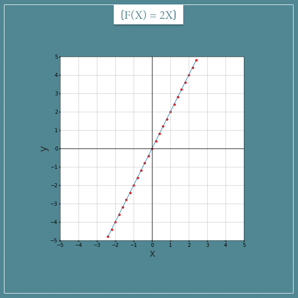
The blue line is the actual plot of the function in that interval. It represents infinitely many points next to each other. The red points are just random samples highlighted to emphasize that the line consists of points.

Let’s look at another example. Say we have the function . That is, one that takes any real number and returns its square. Here’s what the plot looks like on the same interval:

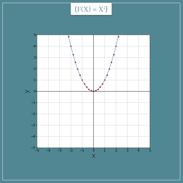
Notice that negative real numbers are not part of the range here, since any number’s square is positive or zero.

Finally, let’s look at the graph of the function :

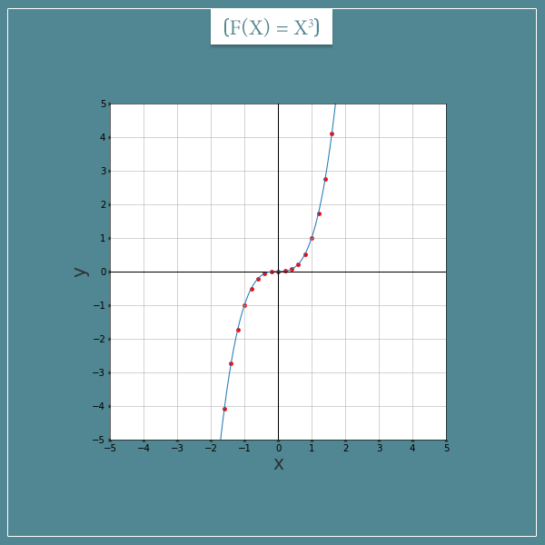
See how plotting even a small interval from the domain gives a pretty good idea of what a function looks like as a whole?

Important concepts and properties

In this final section I want to introduce a few important concepts and properties related to functions which will improve your intuition for them.

Injective, surjective, and bijective functions

Let’s look again at the CountryLanguage function from one of the earlier sections:

I drew your attention to the fact that some elements in the codomain are reached by more than one element in the domain. Now compare this to the function:

Here every element in the codomain is reached by exactly one element in the domain. For example, the element 6 in the codomain maps to the element 3 in the domain and no other element in the domain maps to 6 in the codomain.

This leads to the first important property. A function is called injective if every element in its codomain is related to at most one element in its domain. Another name for the injective property is one-to-one, which probably sounds more intuitive. So, based on this property, is injective, whereas CountryLanguage is not.

Now take a look at the CountryLanguage function again. Earlier I also drew your attention to the fact that its range is a proper subset of its codomain. That is, it has elements in the codomain that will never be reached. And hence, never returned as outputs. On the other hand, the range of is the same as its codomain (namely, the full set of real numbers). To get to any element in the codomain, simply divide it by two and you will find the corresponding element in the domain.

Well, functions with the property of having the same set as both their range and their codomain are called surjective or onto. Again, according to this definition, is surjective and CountryLanguage is not.

Finally, a function is bijective if it is both injective and surjective (obviously, satisfies this definition). Another name for a bijective property is invertible. Which brings us to the next concept: the inverse of a function.

(As an exercise, try to determine if the remaining function examples I showed you earlier are injective, surjective, or both.)

Inverse of a function

The concept of an inverse of a function is very simple and intuitive. To invert a function basically means to turn its domain into codomain and its codomain into domain. You keep the same associations between elements as before, only you reverse the directions of the arrows.

Importantly, the only functions with which you can do this are bijective functions. Let’s immediately look at an example. We already know that is bijective. To invert it, we simply need to invert the following relationship by solving for x:

   

Which we can do by dividing both sides of the equation by 2 to get:

   

Let’s plot this:

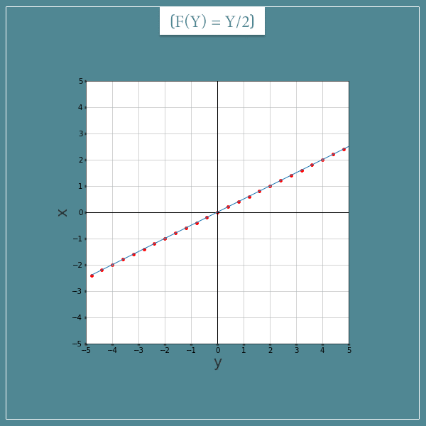
Notice the relationship between the graphs of and . Basically, one is just a rotated version of the other. Yep, inverting functions is as simple as that.

A common notation for the inverse of a function is:

   

It looks like the function raised to the power of -1, but this is more an overlap in notations (don’t think about it as an actual power). For those of you who read my introductory post on arithmetic operations, this is analogous to the notation for the multiplicative inverse of a number

Speaking of which, you might also see a direct connection between the inverse of a function and the inverse of an arithmetic operation. We’re going to explore this relationship in more depth in one of my next posts where I’m going to show you the most common families of mathematical functions.

Why only bijective functions are invertible

Now, do you see the problem with inverting functions that aren’t bijective?

For example, consider a function that is not injective (not one-to-one). Well, is a good example because every value in its range maps to exactly 2 values in the domain (except for 0, which maps only to 0).

For example, 4 maps to both 2 and -2, since the square of both is 4. If we tried to invert , what output will produce, 2 or -2? Remember, a function should give a unique output for each input in its domain! So, you see the problem here.

What if the function is not surjective? This means that some elements in its codomain aren’t associated with any element in the domain. Take the CountryLanguage function, for example. If we tried to invert it, what would be equal to? Latin is currently not the most common language in any country, so the function won’t be able to produce any output. And this is not allowed, because a function is supposed to be able to give an output for every element in its domain.

So, to summarize, a function is invertible if and only if it’s bijective. Which means that its range must be equal to its codomain and every element in the codomain must be associated with exactly one element in the domain.

Composing functions

Alright, the last concept I want to talk about in this post is function composition. This is also a pretty simple and intuitive concept related to chaining different functions together.

Until now I was using the function name f almost exclusively, even in the same context. This isn’t exactly accurate but I did it because I didn’t want to introduce too many different function names. But here we need to do that.

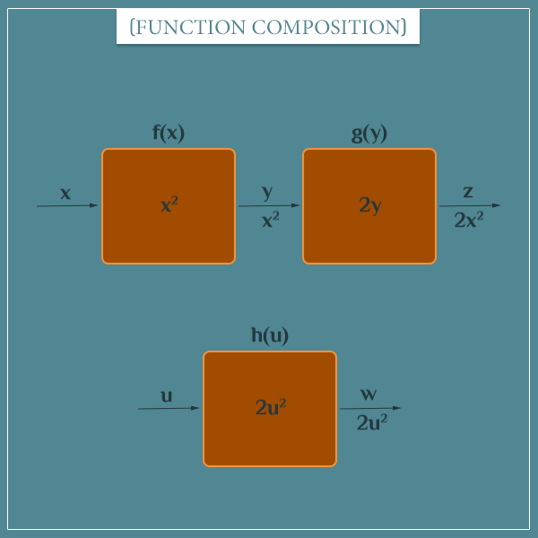
So, consider two functions, f(x) = y and g(y) = z. What if we define a third function, h(u) = w, which is the combined effect of f and g? Here’s what I mean.

The match in names of the output variable of f and input variable of g isn’t a coincidence. In this example, we’re assuming that the codomain (or at least the range) of f is a subset of the domain of g. So, imagine we take the outputs of f and pass them through g. This is all that function composition is!

Let’s consider two concrete functions to see what I’m talking about:

   

   

Now let’s pass the output f to g:

   

You see that the combined effect of f and g can be produced with a single function like so:

   

Take a look at this diagram for some visual intuition:

Another common notation for function composition is:

   

You can, in principle, chain as many functions as you like. For example, this is a composition of 3 functions:

   

But notice that the order matters here. In the general case:

   

For example, if:

   

   

Then:

   

   

In other words, function composition is not commutative! Well, this is a good opportunity to tell you that the commutative property I showed you in the context of arithmetic operations is actually a more general mathematical property. But we’ll talk about this in more detail in future posts.

A small exercise

With all this in mind, let me ask you a question. What do you think the following expression is equal to?

   

Or, alternatively:

   

While you’re at it, try to find what this expression is equal to as well:

   

This is a simple exercise that will help you in building your intuition about functions.

Summary

In today’s post, I introduced you to mathematical functions. They are a special type of a relation between two sets, the domain and the codomain. More practically, a function is an input-output machine. One which accepts inputs from one set (the domain) and associates each input with a specific output from another set (the codomain). The subset of the codomain which includes the actual output values is its range.

The set of all input-output pairs of a function is called its graph. Using a graph, we can plot a function on a Cartesian plane (by plotting the elements of the graph as points).

I also introduced the injective, surjective, and bijective properties. Injective functions are those which associate at most one domain element to every codomain element. On the other hand, surjective functions are those whose range and codomain are the same set. And bijective functions are those which are both injective and surjective.

And I also introduced the inverse of a function, denoted as , which simply reverses the direction of the associations. That is, the inputs become the outputs and vice versa. I also explained why only bijective functions have inverses.

Finally, I told you about function composition which is taking one value and passing it through 2 or more functions, where the output of the previous function in the chain becomes the input of the next function. The notation here is , which means to first pass the value through the f function and then pass f’s output to g. I also told you that order matters and most of the time .

In one of my next posts, I’m going to show you some commonly used functions and their properties. As always, if you have any questions or comments, you’re welcome to share your thoughts in the comment section below!