The Mean, the Mode, And the Median

The concepts of mean, median, and mode are fundamental to statistics, probability theory, and anything related to data analysis as a whole. Being this important, they deserve their own introduction.

In statistics, these 3 concepts are examples of measures of central tendency. This is a fancy way of saying that they are single values that summarize collections of values.

Let’s unpack the last sentence. What exactly do I mean by ‘values’ and ‘collections of values’?

Table of Contents

Values and collections of values

Values are simply numbers, like 5, 1, 3.6, 1041, 0, 200, 0.5, -100, etc. Of course, in data analysis you often deal with vectors, but here I’m going to ignore them for 2 reasons. First, introducing vectors is beyond the scope of this post and would unnecessarily complicate things. Second, even though generalizations of the mean, mode, and median to higher dimensions do exist, they aren’t necessarily unique. So, from now on, instead of values, I will simply refer to them as numbers.

What do these numbers stand for then? Well, they can stand for pretty much anything. Each number could represent the height, weight, age, income, IQ score, etc. of one person. Or it could stand for counts of traffic incidents for a particular country, daily temperatures in a particular city, and so on.

In this context, a collection of values is simply a list of numbers that are related in some way. For example, you could have the list of all student heights in a particular school. Or the count of traffic incidents for a particular year for each city in a particular country.

From now on, I’m going to express collections of numbers as lists inside square brackets, like: [4, 12, 9, -4, 222].

With this out of the way, let’s see the kind of numbers that the mean, the mode, and the median are.

Measuring central tendency

Say we’re looking at heights of people (in cm) and we have the following collection:

[193, 201, 185, 205]

Your first impression might be that, whoever these 4 people are, overall they are rather tall. Why? Because to you any height greater than (say) 180 cm means the person is tall and everybody in that list meets this criterion.

On the other hand, if the collection is:

[165, 150, 154, 166, 150]

This time your impression is that the people represented by these heights are overall short.

I underlined the word overall twice because this is an informal way of expressing the idea of a central tendency — some way of describing the entire collection in a few words. If the values are just 4-5, you can easily list them all and that would still give a good “summary” of the collection. But if the values are 1000 or more and you still want to give a summary of the entire collection, listing all numbers would be more than impractical.

“Just take the average of all numbers!” you say. That’s correct. “Taking the average” refers to calculating the (arithmetic) mean of all numbers. It’s one of the most common measures of central tendency in statistics, but it’s not the only one. The mode and the median are also measures of central tendency and each is a way of summarizing a collection of numbers, just like we did verbally with the word “overall”.

But unlike the vague description of “overall”, means, modes, and medians have precise mathematical definitions (and properties that follow from those definitions).

Without further ado, let’s look at how these measures are calculated.

Calculating the mean

NOTE: There are other measures of central tendency with the term ‘mean’ in their name, such as harmonic mean and geometric mean. But in this post, by ‘mean’ I will only be referring to the concept of arithmetic mean.

The mean is very simple to calculate in 3 steps:

Sum all numbers in the collection.
Count the numbers in the collection.
Divide the sum by the count.

For example, the mean of the first example collection of heights [193, 201, 185, 205] is:

$\frac{193 + 201 + 185 + 205}{4} = 196$

Similarly, the mean of [165, 150, 154, 166, 150] is:

$\frac{165 + 150 + 154 + 166 + 150}{5} = 157$

You see, the collection which we said had “overall tall people” in it has a mean of 196 cm. This is indeed considered a high value for humans. And the mean of the “overall short people” collection is 157 cm, which is considered low for adults. So, the mean does seem like a good way to capture a central tendency of a collection.

Calculating the median

Calculating the median is also very simple, though it requires a bit more work. Here are the steps:

Sort the collection of numbers in an ascending order.
Find the middle number of the sorted collection.
1. If there’s an odd number of values in the collection, get the value exactly in the middle.
2. If there’s an even number of values in the collection, get the mean of the two middle values.

In other words, the median is that number which is greater than half of the numbers in the collection and less than the other half.

For example, to calculate the median of [165, 150, 154, 166, 150], we first sort the collection:

[150, 150, 154, 165, 166]

Since the count of numbers is odd (5), the median is the middle number 154.

Similarly, to calculate the median of [193, 201, 185, 205], we first sort the collection:

[185, 193, 201, 205]

Because there are only 4 numbers and the count is even, the median is the arithmetic mean of the two middle numbers 193 and 201, which is 197.

Easy enough, isn’t it. But is the median a good measure of central tendency?

For the “tall” collection, we got 197 cm, which is again a number that does represent “tallness”! (compare this to the mean of this collection, which was 196 cm.)

For the “short” collection, the median is 154 cm, which is also a good representative number for “shortness” (and is also close to the mean of 157 cm we calculated earlier).

In both examples, the calculated means happened to be very close to the calculated medians. But this isn’t always the case, as I will show in a bit.

Calculating the mode

Of the three measures of central tendency I’m introducing in this post, the mode is probably the easiest to calculate. It’s the value in the collection which appears the highest number of times.

For example, the mode of [165, 150, 154, 166, 150] is 150, because 150 appears twice, whereas all other numbers appear only once (compare to the median of 154 and the mean of 156).

On the other hand, the collection [193, 201, 185, 205] doesn’t have a mode, because each number appears only once. This is generally true for all collections where each number appears an equal number of times. Here’s a few other examples of collections that don’t have a mode:

[2, 6, 9, 9, 5, 7, 6, 7, 5, 2]
[1, 2, 1, 1, 2, 2]
[5, 5, 5, 4, 5, 4, 4, 4, 3, 3, 3, 3]

An exception to the above case is if you have only one number in the collection (even if it doesn’t repeat). Then the mode exists and is equal to that number. For example the modes of these 3 collections are, respectively, 1, 8, and 13:

[1, 1, 1]
[8]
[13, 13, 13, 13, 13]

A third case is where you have 2 or more numbers in the collection with an equal maximum count. In such cases, more than one mode exist. For example, the collection [1, 1, 1, 4, 7, 3, 2, 2, 2] has 2 modes: 1 and 2 (each appears 3 times). The collection [33, 9, 33, 5, 5, 2, 2, 7] has 3 modes: 2, 5, and 33 (each appears 2 times).

Properties of the measures of central tendency

Calculating these measures of central tendency is easy but which should you choose? And, once you calculate it, how exactly should you interpret its value?

To start this discussion, first notice the obvious: when you use either of these measures to “summarize” an entire collection, you lose information about individual numbers in the collection. In a way, reducing an entire collection to a single number is like data compression. But unlike some forms of compression you’re used to (like “zipping” the files on your computer), here a lot of information is lost because you cannot recover the original collection from the calculated measures of central tendency.

So, for these measures to be good summaries of a collection, they better carry enough information about the individual numbers. As you can potentially have a lot of numbers, it seems like this is already asking too much from a single measure!

For this reason, it’s important to understand the kind of information you lose when using each of them. More generally, it’s important to know the properties of these measures, in order to know which might be more appropriate for a particular collection of numbers you’re interested in.

The mean, the mode, and the median running for president!

Imagine 3 candidates running in some election. Each candidate is trying to convince you to vote for them by promising to represent you better than the other 2 candidates. Of course, the candidates aren’t trying to convince only you. In fact, to maximize their winning chances, they want to convince as many voters as they can. Hence, they want to be representative of as many voters as possible. In the end, the best overall representative of the voters will win the election.

Let’s use this scenario as a metaphor for our 3 measures. For any particular collection of numbers, the mean, the mode, and the median will be values that represent the collection as a whole. How well do they represent it? For which collections of numbers should each measure be preferred?

In the following sections I’m going to discuss some of the main properties of each measure. I’m going to show that how “representative” they are of a particular collection depends on the kind of collection we’re dealing with.

From here on, I’m going to use the following notation:

x = a particular real number
S = the sum of all numbers in a collection
N = the count of numbers in a collection
MEAN, MODE, MEDIAN = the respective calculated measures for a collection

In the spirit of the election metaphor, let’s hear the arguments in favor of each measure and see which one we should choose!

A warm-up simulation

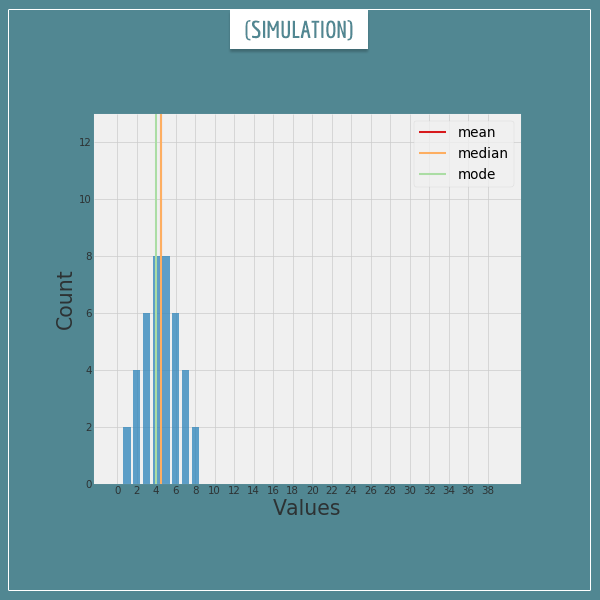
A simulation is a good way to get an intuition for how the 3 measures behave. Let’s start with an innocent looking collection of numbers whose mean, mode, and median are all in the middle.

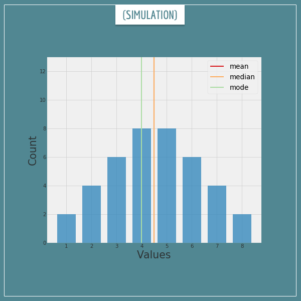
The x-axis represents individual numbers in the collection and the y-axis shows how many of each number there is.

The red, orange, and green lines indicate the current values for the measures. The first 2 are both equal to 4.5, whereas the latter is equal to 4 (the red and orange lines are currently overlapping and that’s why you can’t see the red one).

Let’s make some room on the right and start adding new numbers to the collection. After each number, the central tendency measures will be recalculated and their lines moved to the new values. Click on the image below to start this simulation.

Click on the image to start/restart the animation.

First impressions?

For one thing, as new numbers arrive, the mean is the first to “notice” them and start moving in their direction. Meanwhile, the other 2 mostly remain where they are.

At some point, when the new numbers become too many, the median and the mode switch sides and jump to where the majority of the numbers are, while the mean is not so quick to abandon the initial collection.

Also worth noting is the “smoothness” with which the measures change. The mean always slides continuously along the x-axis. The median, on the other hand, likes to either wait or jump abruptly from one number to its neighbor. The mode is even more chaotic in its behavior, as it stays in one place most of the time but can abruptly jump to a completely different position.

Let’s dig deeper into each measure to see the root of these behaviors.

The mean

Consider the following 2 collections:

[3, 4, 5]
[4, 4, 4]

For both we have N = 3, MEAN = 4. Notice that the second collection has the same element (x=4) repeated N times and the mean happens to be that very element. That is, MEAN = x, which is obviously going to hold true for any N and any x, as long as x is the only element in the collection.

Then, in a way, using the mean to describe a collection of numbers is a bit like reducing the collection to a corresponding collection with the same N but where every element is replaced with the calculated mean.

So, if we choose to represent the collection [3, 4, 5] by its mean, it’s as if we are actually representing it as the collection [4, 4, 4]. How good is this representation? Not too bad. The numbers 3, 4, and 5 are all very close (or identical) to the mean of 4.

Now let’s consider the collection [-94, -58, 164]. The mean here is also (-94 + (-58) + 164) / 3 = 4 and so this collection is also reduced to [4, 4, 4]. Let’s compare it to its candidate representative:

[-94, -58, 164]
[4, 4, 4]

Does the mean still seem like a good representative for the individual values in the collection? Not so much.

The point I’m making with this is that, when considering if the mean adequately represents a collection of numbers, a good starting point is to always imagine how the collection compares to a reduced version where all values are equal to the mean. Incidentally, you use the same line of reasoning for the other two measures as well.

The mathematical intuition behind the mean

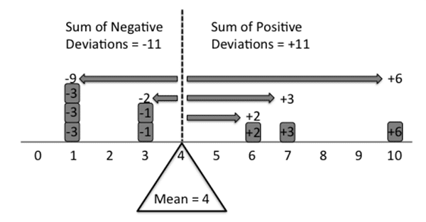
Let’s look at another collection, [1, 1, 1, 3, 3, 6, 7, 10], whose mean is also equal to 4. I’m borrowing this example and the following visualization from Watier, Lamontagne, & Chartier (2011):

Notice that, for each x in the collection, there is a corresponding difference d = x – MEAN. If x is less than the mean, d will be negative, if x = MEAN, d will be zero, and if x > MEAN, d will be positive.

So, imagining each d as a weight, the mean is that number which exactly balances the sums of positive and negative weights.

The mean’s sensitivity to new values

Let’s consider what happens to the mean when we add a new number, x, to the collection. If x is equal to the mean, the new mean will be equal to the old one, since you’re not adding a positive or a negative d on either side of the “scale”. But if x is not equal to the mean, you will now have to shift the new mean to the left or to the right, in order to balance the new list of differences.

A natural question is, how different can the new mean be from the old one after adding a single new number to the collection?

The old mean is equal to the sum of the numbers divided by their count:

$MEAN_{old} = \frac{S}{N}$

For the new mean, we’re adding a new value x and the new sum becomes S+x, whereas the new count becomes N+1:

$MEAN_{new} = \frac{S+x}{N+1}$

The absolute difference between the two means is:

$\left | MEAN_{old} - MEAN_{new} \right | =$

$= \left | \frac{S}{N} - \frac{S+x}{N+1} \right |$

$= \left | \frac{S - N \cdot x}{N \cdot (N+1)} \right |$

$= \left | \frac{S}{N \cdot (N+1)} - \frac{x}{N+1} \right |$

$= \left | \frac{MEAN_{old}}{N+1} - \frac{x}{N+1} \right |$

$= \frac{\left | MEAN_{old} - x \right |}{N+1}$

Since at any given moment N is a constant, we can ignore the denominator in the last expression. Notice that, no matter what the value of MEAN_old was, a new x can pull the new mean arbitrarily far away from the old one, as long as x is small/large enough. Not only that, it can pull the new mean arbitrarily far from the entire original collection!

How well does the mean represent the collection?

Think about the implications of this finding. Even if a mean is a very good representative of all values, adding a new value to the collection which is too “far away” from the existing ones (commonly referred to as an ‘outlier’) will force the mean to shift to a new point where now it will be “far away” from all values!

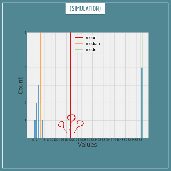
Look at the example above. Here we have the bulk of the collection around the values 1 through 5. We also have four outlier values far to the right of the bulk. The median has stayed with the bulk and the mode has jumped all the way to the outliers. The mean, on the other hand, has shifted somewhere to the middle. This is an attempt to find a “fair compromise” between all values. But, where it stands, who is it actually representing…? Well, nobody.

With all this in mind, feel free to go back and re-watch the simulation above. Does the behavior of the mean make more sense now?

The median

One way to think about the behavior of the median is that it doesn’t care how far away it is from individual numbers in the collection. It’s happy as long as it splits the collection right in the middle.

This explains why in the simulation above it took so long for it to move significantly far from its original position. Adding a single number anywhere to the left or to the right of the median simply increases the total count of numbers on that side by 1. Hence, most of the time the median will need to move very little to accommodate this new number.

You might have heard that medians are much less sensitive to outliers compared to means. Well, now you see why — by definition, an outlier is a value which is far away from the bulk of the collection. But we just saw that the median hardly cares about how far away from it individual values actually are!

One consequence of this behavior relates to how much the median can change after adding a new number to the collection. Remember that if the new value is extreme enough, it can pull the mean arbitrarily far away, even outside the range of the original collection. But the new median can never go outside the original range. In fact, the most it can change is by 1/2 of the original range, in extreme situations like when you have this collection:

[0, 0, 100]

The median is currently 0, but if you add a new value of 100:

[0, 0, 100, 100]

The new median will be 50.

While jumps equal to 1/2 of the original range can happen, they are rare and most of the time the new median will shift much less.

The mathematical intuition behind the median

To give a better understanding of the median, I first want to introduce a generalization of the mean, called the truncated mean. The truncated mean of a collection is simply the mean calculated after excluding some numbers from the extreme ends. How many numbers to exclude can be indicated as a percentage of the total count or as a fixed integer. The common practice is to exclude equally from both ends of the collection.

Let’s again look at the collection [1, 1, 1, 3, 3, 6, 7, 10]. In this case it happens to be sorted, but if it wasn’t we would have had to do it ourselves. As we know, its mean is 4.

Now, let’s remove 1 value from the left and from the right. The new truncated collection is [1, 1, 3, 3, 6, 7], with a mean of 3.33.

Truncate it again: [1, 3, 3, 6] with a mean of 3.25.

And again: [3, 3] with a mean of 3.

We can’t truncate anymore, as that would leave no numbers in the collection. But do you notice something? The most extreme case of the truncated mean (3) is actually equal to the median of the collection!

In fact, this holds true for any collection. You keep calculating the truncated mean after excluding more and more values from both side. The last possible truncated mean will be equal to the median of the original collection. Pretty neat.

Now it should be even more obvious why medians are insensitive to outliers. Those are all “thrown away” in the process of calculating the median!

The mode

Since the mode only cares about which number in the collection is most frequent, there’s hardly any mathematical intuition to be shared here. For most collections, the mode will be the worst choice for representing it, as it loses information about all other numbers.

This behavior of the mode explains why it erratically jumps between values, even if the values are very far from each other. In a way, the mode’s behavior is very consistent, but not too reliable.

The mode will be a good representative of a collection when the collection is dominated by one specific number, with the occasional exceptional values here and there. In other words, unless you have an extremely homogeneous collection of numbers, avoid using the mode as the only measure of central tendency.

Another serious problem with the mode is that, like I showed earlier, often you can have 0 or 2 or more modes, which renders this measure rather unusable in those cases.

Summary

Earlier I said that it’s important to understand the kind of information you lose when using each of the three measures. After the observations and analyses in this post, we can summarize what each measures misses from a collection:

The mean doesn’t know the region where the bulk of numbers are located. It only knows that it exactly balances the sums of distances of all numbers from itself.
The median doesn’t know how far away the numbers are from it. It only knows that it splits them exactly in the middle.
The mode doesn’t know anything about any number in the collection but the one which appears most frequently.

To be a good representative of a collection, a single value must be “similar” to as many numbers in the collection as possible. This is another way of saying that a measure of central tendency should “look like” the typical value in the collection.

With all these considerations, you can have better judgment regarding the use of each measure as a summary for collections of numbers.

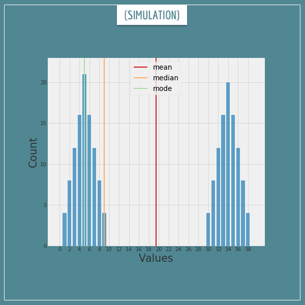
Sometimes you might have a collection for which none of the measures would be a good choice, such as this one:

Here, the mean is in the middle of nowhere. The median is at the extreme end of the left part of the collection. The mode is stuck on the most frequent value, as usual ignoring everything else. None of the three values can be safely chosen as good representatives of the “typical” number in the collection.

Sometimes a single measure just isn’t enough.

Final words

In this post, I have skipped a few important topics.

First, the (arithmetic) mean, the mode, and the median are not the only measures of central tendency in existence. In the beginning I mentioned the harmonic and geometric mean, but there are many others.

Second, I have been referring to the numbers as a collection. A more appropriate statistical term would be a sample. Throughout this post, I’ve been implicitly assuming that we’re dealing with samples, and not probability distributions (both discrete and continuous). To learn about calculating the mean of a probability distributions, check out my dedicated post.

Third, I haven’t discussed the higher dimensional versions of these measures (when the values in the collection are vectors).

Last, but not least, I haven’t mentioned anything about measures of dispersion. Most of you have heard of the most common one, the variance.

While important, these topics are beyond the scope of the current post. My main goal here was to give an intuitive understanding of the kind of information about a collection these measures hold. And, hopefully, to help you make good decisions for summarizing your own data, as well as to have a proper judgment when reading other people’s statistical reports!