The Inverse Problem and Bayes’ Theorem

The inverse problem is fundamentally related to the subject of causality. Think about a scenario…

What will happen if you grab a solid rock and throw it at your neighbor’s window? The most common result is that the window will break. If your neighbor later asks if you know anything about the incident, you can confidently inform him that his window was broken because you threw a rock at it earlier. Cause and effect — sounds pretty straightforward.

But what if it wasn’t you who broke the window and, in fact, you have no idea what broke it? Did someone else throw a rock at it? Was there a large temperature difference between the center and the periphery of the glass which caused a spontaneous breakage? Or was it a spontaneous breakage caused by a fabric defect?

You see, unlike the previous question, this one is actually not straightforward to answer. It involves solving the sо-called inverse problem: inferring the causes of a particular effect.

In this post I’m going explain the inverse problem and give two examples of how it shows up in nature and science.

Bayes’ theorem is a powerful method for addressing the inverse problem in general. In the last section of the post, I’m going to demonstrate how to do this with a toy example. If you aren’t familiar with Bayes’ theorem, go ahead and check my introductory post.

The forward and the inverse problems

In science, solving the forward problem means trying to predict the effects of a particular cause. Examples of questions that address the forward problem are:

• In which direction will a piece of magnet move if there is another piece of magnet next to it?
• How will the color of a litmus paper change if you put lemon juice on it?
• How will the structure of a glass window change after an impact with a rock of a particular mass and velocity?

Most of the time, the forward problem is well-posed.

In mathematics, a well-posed problem is one which has the following 3 properties (first suggested by the French mathematician Jacques Hadamard):

1. The problem has a solution.
2. The solution is unique.
3. The solution is dependent and sensitive to the details of the problem.

The last property basically means that small changes in the details of the problem should only require small adjustments in its solution.

A problem which lacks either of these properties is called… ill-posed. You can see how trying to solve an ill-posed problem will generally make your life more difficult than solving well-posed problems.

To solve an inverse problem means inferring the causes of a particular effect. For example, if you see a moving magnet and want to find the cause of its movement (another magnet? strong wind?), you would be solving the inverse problem.

Most of the time, the inverse problem is ill-posed because it lacks the second of Hadamard’s properties. More than one cause can explain most effects. In fact, very often an infinite number of possible causes can explain an effect.

To summarize:

• The forward problem is predicting the effects of a particular cause. A forward problem is often well-posed.
• The inverse problem is finding the causes of a particular effect. Most of the time it’s ill-posed.

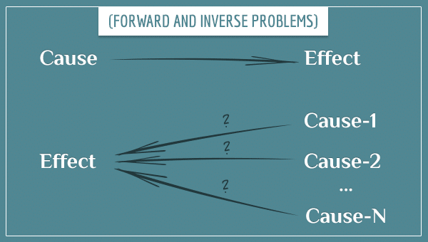
The fact that inverse problems are ill-posed doesn’t mean attempting to solve them is a hopeless effort. You can solve them indirectly (but not necessarily completely) with the help of additional information you use to narrow down the possible causes of an effect.

Inverse problem examples

In this section, I’m going to show two examples of where you can encounter the inverse problem.

Visual perception

When processing information, your brain is constantly trying to solve problems that fall in both forward and inverse categories. An example of the latter is visual perception. Think about how you perceive the correct size and distance of different objects in the environment, for example. You can’t do it directly because a small square 1 meter away from you will look exactly the same (will have the same retinal projection) as a larger square, say, 10 meters away from you.

Yes, they really look the same: your brain receives identical visual input for objects of different sizes, as long as they are at the right distance from your eyes (this follows from pure optics). This means that there is an infinite number of candidates for the right size and distance of any object.

How the brain solves the inverse problem

As I mentioned before, you can solve an inverse problem indirectly with the help of additional information. The brain actually uses two sources of such information:

1. Prior information about the object. You brain has expectations for the typical sizes of many familiar objects, like cats, people, cars, trees, smartphones, and so on. These expectations come from past experience. So, after seeing an object, your brain assumes it has the typical size as other objects from the same category. Once the size of an object is fixed, inferring the distance becomes a well-posed problem and can be solved directly.
2. Contextual information from the surroundings. If you’re looking at an unfamiliar object, your brain will make a guess about its size and distance using cues from the surrounding environment (like the size and distance of familiar objects around it). For example, if you see a person standing next to an unknown object, your brain will infer the size of the object by comparing it to the size of the person (for which it already has an estimate from past experience).

Most of the time, your brain uses both sources. When you look at the details, the process is actually much more complicated than I make it sound.

Funny things happen when these two sources give conflicting information. The Ames room is a famous example of an optical illusion caused precisely by your brain’s attempts to resolve such conflicts. Take a look at this 1-minute demonstration and explanation of the effect by the neuroscientist Vilayanur Ramachandran:

Most of the time the brain solves the inverse problem almost perfectly and almost immediately. However, as the example above shows, this is not always the case and you can trick a brain into solving the problem in a wrong way.

EEG recordings

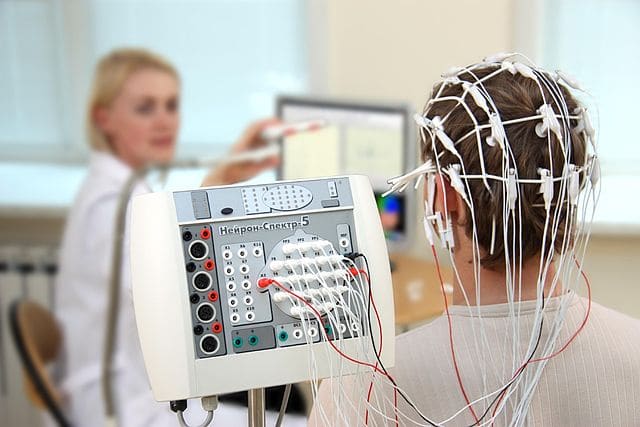
The inverse problem also commonly appears in science when inferring the possible sources of particular measurements. An example of this is interpreting EEG measurements of brain activity.

The white electrodes placed on the scalp are there to pick up the electric potentials generated by the activity of large groups of neurons in the brain. The goal is to use the recordings on the scalp to infer things about the underlying brain activity (like which regions are responsible for it).

This problem is very similar to the one in the visual perception example: there’s an infinite number of possible brain activity patterns that can produce the electric potentials recorded on the scalp. However, that doesn’t mean that all of these patterns are equally plausible. To infer the most likely brain sources of the recorded activity, scientists in the field have developed mathematical techniques that rely on certain implicit or explicit constraints (the “additional information” needed to address inverse problems).

Solving inverse problems using Bayes’ theorem

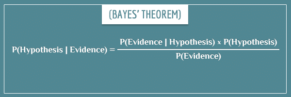
When you have many possible hypotheses for the causes of a particular effect, the problem of finding the correct one becomes probabilistic in nature. This makes Bayes’ theorem a perfect tool for solving an inverse problem.

What you have to do is collect evidence and apply Bayes’ theorem to update the probability of each hypothesis:

A job whose description is almost synonymous with “solving inverse problems” is that of a detective. The job requires investigating cases where there is an observed effect (usually a crime) of an unknown origin. To solve a case means to find its most likely origin. So, in this section, I’m going to show how you can use Bayes’ theorem for solving an inverse problem with a toy detective example.

A detective applying Bayes’ theorem to solve a case

Imagine that you’re a detective and you’re investigating a case of a gas station robbery. After interviewing a few witnesses, you’re certain about the following:

1. The robber was wearing a brown t-shirt.
2. He had a goatee.
3. He escaped on a motorcycle.

Lucky for you, there are only 3 suspects:

1. Jon
2. Bob
3. Tim

So, you build a hypothesis for each of them:

• Hypothesis-1: Jon robbed the bank.
• Hypothesis-2: Bob robbed the bank.
• Hypothesis-3: Tim robbed the bank.

For convenience, I’m going to label the three hypotheses simply “Jon”, “Bob”, and “Tim”.

Example probabilities

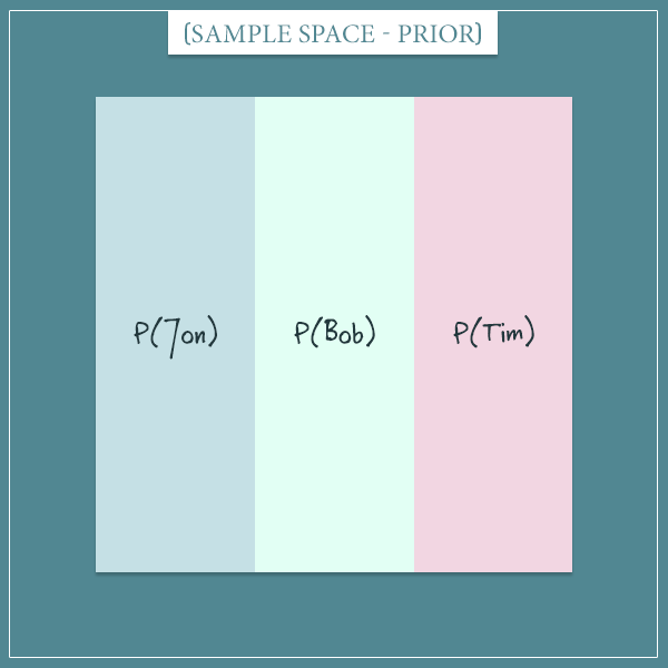
Because you initially don’t know anything about the suspects, you assign them equal prior probabilities:

   

   

   

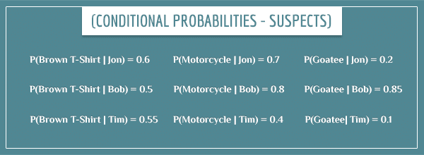
Your goal is to use Bayes’ theorem to update those priors with the 3 pieces of evidence you collected from the witness interviews. In order to get the posterior probabilities, you need to know how the 3 hypotheses predict each piece of evidence. In other words, you need the values of the conditional probabilities:

• P(Goatee |  Jon)
• P(Motorcycle |Tim)
• P(Brown t-shirt | Tim)
• Etc.

Normally, estimating a conditional probability like P(Goatee |  Jon) is difficult. You would need to take into account information like:

• Whether Jon has a goatee now.
• If not, analyze his face to see if there are any  recent shaving marks (in case he shaved after the day of the robbery to cover himself).

But, because this is a toy example, I can assign any values to those probabilities I want:

If the posterior probability term represents the solution of an inverse problem, the likelihood term represents the solution of a forward problem. It is the probability of observing the effect you are trying to explain if the hypothesis whose posterior probability you’re calculating is true. This is an important point because it shows the relationship between forward and inverse problems.

Alright, now all the information necessary for calculating the posterior probabilities is available. If you have any difficulties following the next steps, check my post Bayes’ Theorem: An Informal Derivation where I explained the mathematical theory and the intuition of Bayesian calculations.

Calculating the posterior probabilities

So, initially the sample space is uniform because each hypothesis has the same probability:

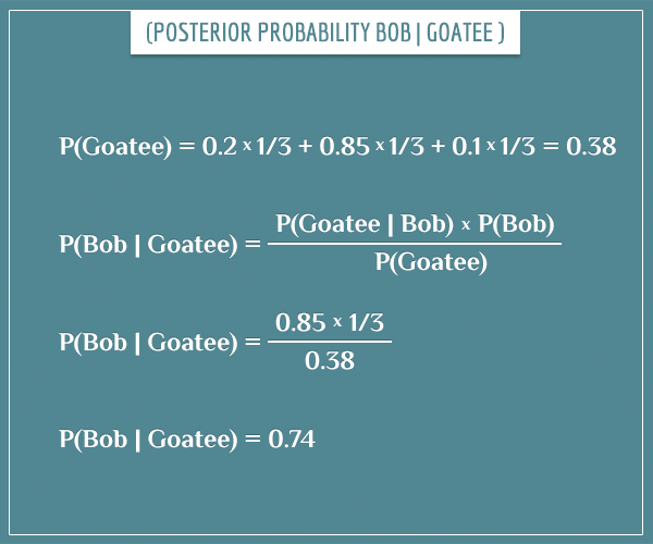
To calculate a posterior probability like P(Bob | Goatee), you need the values of the prior probability, likelihood, and evidence terms. The first two are already available and the evidence term is the sum of the prior probability*likelihood pairs for all hypotheses (capital G stands for “goatee”):

   

Here’s the actual calculation of P(Bob | Goatee):

Applying this to the remaining two hypotheses gives you the following posterior probabilities:

   

   

   

And the new sample space is:

A big difference compared to the prior sample space! The reason the odds turned so much in favor of Bob is that the likelihood term P(Goatee | Bob) was much larger compared to that of the other suspects. Intuitively, the fact that there was a high probability that Bob had a goatee during the robbery increases the chance that Bob was the robber, given that you know the robber had a goatee.

Re-updating the new priors

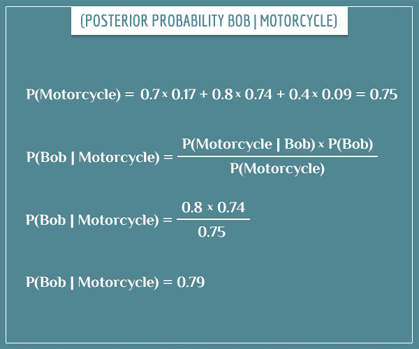
Here’s the cool part: these posterior probabilities become the new prior probabilities which the next piece of evidence can update. For example, here’s how you calculate P(Bob | Motorcycle):

Here are the values of the new posterior probabilities:

   

   

   

Not a huge shift this time, although P(Bob) still increased at the expense of the other two hypotheses. Notice the prior probabilities P(Jon), P(Bob), and P(Tim) used in the calculation were no longer equal to 1/3, but to their respective posterior probabilities calculated in the previous step.

Applying the same procedure to the last piece of evidence yields the posterior probabilities:

   

   

   

And the final sample space looks like this:

The odds slightly shifted back to Jon, but Bob is still the big “favorite” for being the robber. This is a big increase from to the initial probability of 1/3 (while the other two suspects now seem unlikely robber candidates).

It’s important to point out that here I’m assuming the three pieces of evidence are independent from each other. That is, a conditional probability like P(Goatee | Motorcycle) is equal to P(Goatee).

If you would like to see how to calculate more complicated cases where this assumption doesn’t hold, check out my posts about Bayesian networks (part 1 and part 2) and compound event probabilities. On a related topic, you will likely also find my post on conditional dependence and independence very useful.

Summary

Every time you attempt to infer what caused an observed effect, you’re solving an inverse problem. You encounter inverse problems in physics, chemistry, geology, neuroscience, economics, and probably in every other scientific field in one form or another.

It’s difficult to solve inverse problems because they are often ill-posed and there are many (often infinitely many) possible causes of the very same effect.

Bayes’ theorem is a powerful method for addressing inverse problems by using evidence to update the probability of each possible cause.

Bayesian methods don’t automatically eliminate the difficulties of solving inverse problems. However, even though the solutions are probabilistic and not exact, it allows you to get arbitrarily close to an exact solution. You just have to continue collecting evidence and updating the probabilities of rival hypotheses.