
If you ever took an introductory course in statistics or attempted to read a publication in a scientific journal, you know what p-values are. Оr at least you’ve seen them. Most of the time they appear in the “results” section of a paper, attached to claims that need verification. For example:
- “Ratings of the target person’s ‘dating desirability’ showed the predicted effect of prior stimuli, […], p < 002.”
The stuff in the square brackets is usually other relevant statistics, such as the mean difference between experimental groups. If the p-value is below a certain threshold, the result is labeled “statistically significant” and otherwise it’s labeled “not significant”. But what does that mean? What is the result significant for? And for whom? What does all of that say about the credibility of the claim preceded by the p-value?
There are common misinterpretations of p-values and the related concept of “statistical significance”. In this post, I’m going to properly define both concepts and show the intuition behind their correct interpretation.
If you don’t have much experience with probabilities, I suggest you take a look at the introductory sections of my post about Bayes’ theorem, where I also introduce some basic probability theory concepts and notation.
Table of Contents
P-values and statistical significance
In my post introducing the inverse problem I showed a way to address it using Bayes’ theorem. As a quick reminder, you’re facing the inverse problem when you try to infer the possible cause of a particular set of observations. One way to do that is by forming a hypothesis for each possible cause and then apply Bayes’ theorem to update its probability from additional information.
If you think about it, solving the inverse problem is a big part of the scientific process in general. When scientists make observations in their domain of interest, they want to explain them. Consequently, they form hypotheses for their possible causes and collect evidence to evaluate their plausibility with various statistical methods. As I already mentioned, Bayesian statistics is one of the two major frameworks used for this purpose. The other framework goes by various names:
- Frequentist statistics
- Classical statistics
- Fisherian statistics
The term Fisherian statistics comes from the English statistician Ronald Fisher. However, the framework for hypothesis testing used today is an incidental combination between his approach and that of two other major figures in 20th century statistics: Jerzy Neyman and Egon Pearson.
The rest of this post is dedicated to explaining the logic of the framework. From here on I’m going to use the term Frequentist statistics because I think it’s most representative of the framework’s spirit.
If you would like to know more about the distinction between Frequentist and Bayesian statistics, check out this post where I give a detailed comparison.
Frequentist hypothesis testing
Imagine you want to test the hypothesis that sleeping less than 4 hours impairs people’s memory.
You design an experiment where you randomly divide a number of people in 2 groups. All participants in the experiment learn a list of 100 words from a foreign language and a few hours later go to sleep under your supervision. Then, you wake them up 4 hours (Group 1 participants) or 8 hours (Group 2 participants) after they’ve fallen asleep and ask them to write down as many words from the list as they can remember.
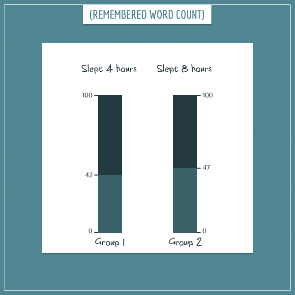
Finally, you calculate the average number of remembered words for each group and you get the following results:
People who slept 8 hours, on average, remembered 5 more words than people who slept 4 hours. Does this support your original hypothesis? Maybe. Consider these possible causes of the observed difference:
- People in Group 2 slept more (your original hypothesis)
- They happened to have better memory skills in general
- People in Group 1 happened to be more distracted while memorizing the list of words
- Some combination of these factors
- Something entirely different
In a Bayesian framework, you would treat this as an inverse problem and calculate the posterior probability of your original hypothesis, given the data from your experiment.
But in the Frequentist framework, you’re not interested in calculating probabilities of hypotheses being true. Instead, you want to calculate the probability of observing the 5-point or greater difference, if you assume that your hypothesis is wrong and there should actually be no difference between the groups.
Pause for a second and read the last sentence again. This probability is at the core of Frequentist hypothesis testing. This is what statisticians in the framework call a p-value.
The null hypothesis
The assumption that the real difference between the groups is equal to zero also has an official term in statistics: the null hypothesis. Тhe p-value is the conditional probability of observing a deviation from the null hypothesis which is greater than or equal to the one you actually observed. In the example above, this would translate to:
Or, in short:
Why would you care about this conditional probability? Is it because a low p-value suggests the null hypothesis is unlikely to be true? And therefore your original hypothesis is more likely to be true?
No. As I said earlier, in the Frequentist framework you’re not in the business of calculating probabilities of hypotheses. Instead, you want to use the p-value to make a decision about rejecting or not rejecting the null hypothesis. Here is the general procedure:
- You come up with some reasonable threshold for rejecting the null hypothesis. The notation used for this threshold is α (the greek letter alpha). This threshold is a real number between 0 and 1 (usually very close to 0).
- You promise to yourself in advance that you will reject the null hypothesis if the calculated p-value happens to be below α (and not reject it otherwise).
The most popular threshold value is 0.05 and was first suggested by Fisher himself. He didn’t really have strong mathematical arguments for choosing this value but it stuck anyway. And to this day, it’s the “official” minimum level of significance for rejecting a null hypothesis (although some fields may require much lower thresholds).
This procedure guarantees that, if you applied it consistently to all null hypotheses that you test, in the long run you will falsely reject at most 5% of the correct ones.
P-values and limiting error rates
Imagine you’re a scientist and you regularly apply the two-step procedure above to test various null hypotheses. In your lifetime you’ll manage to test a certain number of hypotheses. Some of them you will reject and others you won’t.
Here’s a visual metaphor for the list of all null hypotheses you will ever test:
In this image, each small square represents a null hypothesis. Some of these are true and some are false, but you obviously don’t know which ones are which. Every time you “grab” one of the null hypotheses from the “bag”, you go through these steps:
- Specify your α (level of significance).
- Perform an experiment in which you collect data for testing the null hypothesis.
- Calculate the p-value based on the data: P(Data | Null hypothesis).
- If the p-value is less than or equal to α, you reject the null hypothesis. Otherwise, you don’t reject it.
Illustration of the procedure
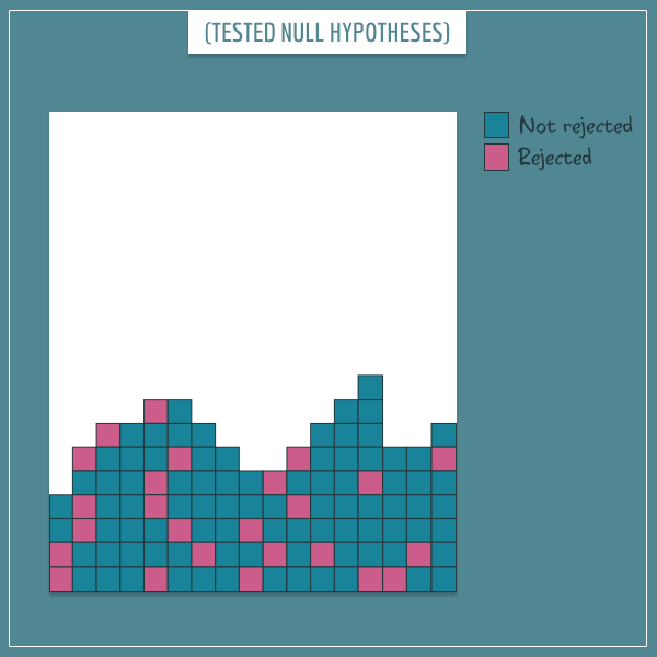
Say you’re in the middle of your career and you’ve managed to test a certain number of null hypotheses. In order to keep track, you color the ones you rejected and the ones you didn’t reject differently. Right after, you throw them in a metaphorical pool of “tested null hypotheses”:
You have rejected some of the null hypotheses and failed to reject others (most of them). Ideally, you want to reject all incorrect hypotheses and leave the correct ones alone. But you will inevitably make some errors in the process.
Your goal is to minimize the 2 types of possible errors that can occur:
- Type I: Rejecting a true null hypothesis.
- Type II: Not rejecting a false null hypothesis.
This is the official terminology used in Frequentist statistics. But you might have come across the same errors under the labels “false positives” and “false negatives”.
The p-value is the probability of the data, given that the null hypothesis is true. Therefore, if you only reject null hypotheses when the p-value is below the level of significance (α = 0.05), in the long run you will falsely reject at most 5% of true null hypotheses you test. So, the p-value, along with the chosen α, directly controls the type I (false positive) error rate.
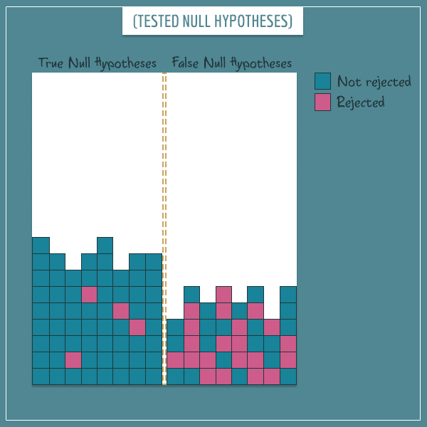
To illustrate what this really does, imagine that there is some omniscient being who knows exactly which null hypotheses are true and which are false. If you asked that being to separate the true from the false ones, the result might look like this:
Examine the last image closely because it’s the most important one in this post.
The type I error
First, focus only on the squares on the left side. They stand for the true null hypotheses among the ones you tested.
You see that you rejected a very small percentage of them. As you continue to test more hypotheses, the number of squares on the left will continue to grow. But the percentage of red squares will never exceed 5% (assuming your calculation of the p-value is correct, of course).
So, the type I error rate is simply:
- The number of red squares divided by the total number of squares.
The type II error
Similarly, the type II (false negative) rate, which is usually denoted with the greek letter β (beta), is the percentage of false null hypotheses that you failed to reject.
Now, only focus on the squares representing false null hypotheses (those on the right). The type II error rate is simply:
- The number of blue squares divided by the total number of squares.
Another way of defining β would be as:
Statistical power
If you count the red squares instead, you get the related concept of statistical power:
In other words, it’s the probability that you will reject a null hypothesis, if it is false.
A question you might be asking yourself is: “If the p-value controls the false positive rate, what controls the false negative rate and statistical power?”. This would actually be a topic for another post but the short answer is that controlling the size of β isn’t as straightforward as controlling the false positive rate. The false negative rate will depend on 3 factors:
- The size of the actual difference between the groups (which, by definition, is nonzero when the null hypothesis is false)
- The variance of the data with which you’re testing the null hypothesis
- The number of data points (your sample size)
In the real world, you only have control over the last factor, so you see why controlling the type II error is much trickier.
P<0.05. So what?
You performed the memory test and discovered people in your experiment who slept 8 hours remembered 5 more words than people who slept 4 hours. Say you calculated the p-value to be 0.035. This is less than 0.05, so you label the 5-word difference “statistically significant” and reject the null hypothesis. What follows from here?
What follows is that the you accept the so-called alternative hypothesis. The alternative hypothesis is simply the opposite of the null hypothesis and says that the difference between your groups is not equal to zero. It doesn’t say how big the real difference is.
This time it happened to be 5 but if you performed another experiment you might get 4, 6, or any other value. These fluctuations are due to random factors like the ones I listed earlier (such as random differences in memory/linguistic skills of people in the two groups). Of course, deviations further away from the real value become less and less likely.
The idea behind this procedure is that you reject the null hypothesis in favor of the alternative hypothesis. And the alternative coincides with the original hypothesis you wanted to test. If you apply this procedure to all hypotheses, and only count a hypothesis as true if you manage to reject the corresponding null hypothesis, in the long run you’ll end up with a type I error rate whose upper bound is α.
Notice that you still know nothing about which specific hypotheses you tested were actually true. In fact, you don’t even know what percentage of the hypotheses you tested were true. These questions are simply not addressed in the Frequentist framework.
This point is extremely important because ignoring it leads to some common misinterpretations of p-values.
Summary
The important concepts I talked about in this post are:
- null hypothesis and alternative hypothesis
- p-value and statistical significance
- type I and type II errors
- statistical power
Based on the hypothesis you want to test, you formulate a null hypothesis which asserts the opposite of your hypothesis. You calculate the p-value and if it’s below a predetermined threshold (α), you reject the null hypothesis in favor the alternative hypothesis.
This procedure controls the long-term type I error rate while also giving the opportunity to limit the type II error rate (β). However, there are no guarantees for the latter because it strongly depends on the size of the effect (deviation from the null hypothesis), if it exists.
This is the gist of it but the real procedure is much more complicated. I haven’t said anything about how p-values are actually calculated. There are many statistical methods for that, depending on the experimental design, the number of groups, the type of hypothesis you’re testing, and so on.
I will cover these and other questions in future posts.

I’d say there is a misrepresentation of the frequentist basis for using p-values. To quote prominent philosopher of science Mayo:
The “P values are not error rates” argument really boils down to claiming that the justification for using P-values inferentially is not merely that if you repeatedly did this you’d rarely erroneously interpret results (that’s necessary but not sufficient for the inferential warrant). That, of course, is what I (and others) have been arguing for ages—but I’d extend this to N-P significance tests and confidence intervals, at least in contexts of scientific inference. See, for example, Mayo and Cox (2006/2010), Mayo and Spanos (2006). We couldn’t even express the task of how to construe error probabilities inferentially if we could only use the term “error probabilities” to mean something justified only by behavioristic long-runs.”
As you can see, referring to long-run performance only as justification for using p-values for inference is something frequentists would staunchly disagree with. More on the topic can be seen in this read on Pearson’s take on the issue of performance versus probativeness: https://errorstatistics.com/2016/08/16/performance-or-probativeness-e-s-pearsons-statistical-philosophy-2/
If you notice, I am neither defending nor criticizing the use of p-values here. Consequently, I don’t really talk about what would justify their use in research or elsewhere.
What is going on mathematically is that the long-run error rates are constrained (well, the type I error rate – type II is a bit trickier). What would you make out of this *philosophically* is a separate question. I honestly don’t think you can make much out of it as a strict Frequentist who refuses to assign probabilities to single events, rather than infinite sequences.
What is revealing for me is the language I often see being used by Frequentists in their attempt to justify the use of p-values. They come up with non-existent words like “probativeness” to describe something that is already well described and, more importantly, *formalized* in the Bayesian framework as “degree of belief” or simply “probability”.
To quote from the article you referenced:
“If we can readily bring about statistically significantly higher rates of success with the first type of armour-piercing naval shell than with the second (in the above example), we have evidence the first is superior. Or, as Pearson modestly puts it: the results “raise considerable doubts as to whether the performance of the [second] type of shell was as good as that of the [first]….” (Ibid., 192)[ii]”
What does it mean for the results to “raise considerable doubts…” if not “the results decrease the probability that the second type of shell is as good as the first”?
The point I was making was not at all about that, but about the fact the a frequentist can reason perfectly well about single “events” that will never be repeated. But, to reply to your comment, anyways:
Yes, it’s necessary to come up with new words for new concepts, same as Bayesians are coming up with new words for “objective” priors: “non-informative”, “uninformative”, “weakly informative”, etc. as they attempt to reach agreement on what these things are and how to describe them in a least-ambiguous way.
In this case a p-value is only a part of the concept of probativeness or “severe testing”/severity as Mayo puts it and I see nothing wrong in using a new term for a new framework of inference. I disagree that it corresponds to a “degree of belief” or a “probability” of a given hypothesis since severity or probativeness is a measure of the statistical procedure, not of any given hypothesis put to test.
You know full well that the second interpretation requires prior probabilities with which severity has nothing to do whatsoever and I believe Pearson knew that better than you and I when talking about his framework. As you say yourself, the p-value is a measure of error probability – type I in this case. A hypothesis is either true or false, probability does not make sense if applied to hypotheses in frequentist terms, where error is attached to the testing apparatus, not the hypothesis being tested.
Since I went back and re-read the article, I should say in light of this there is another issue in it and that is that it presents the p-value as a conditional probability, which it definitely isn’t. It would be quite odd to mathematically condition the probability of some event on a hypothesis being true. One can only condition on things that are random, but a hypothesis is not a random variable or event as it is not something that can happen. It is either true or false in frequentist statistics.
The p-value is in fact a computation of marginal probability of an event given a statistical hypothesis and a statistical model. The error probability is therefore deductively entailed by the probability distribution and the hypothesis in question. Thus the frequentist case should more properly be expressed not as p-value = P(Observation | Null hypothesis), but rather as p-value = P(Observation ; Null hypothesis).
Similarly, for power: P(Reject null hypothesis ; Null hypothesis is false)
There is nothing in the Frequentist framework that assigns probabilities to single events or hypotheses. That doesn’t mean you can’t partially leave the framework and have a hybrid philosophical approach to your data, but that’s the point – you’re out of the framework (without necessarily contradicting it).
But let me ask you this. Is there a mathematical formalization of the concept of “probativeness”, like there is for probabilities in the Bayesian framework? In other words, how do you measure the plausibility of a hypothesis quantitatively?
“I should say in light of this there is another issue in it and that is that it presents the p-value as a conditional probability, which it definitely isn’t. It would be quite odd to mathematically condition the probability of some event on a hypothesis being true. One can only condition on things that are random…”
Both statements are incorrect. You can very much condition on non-random variables and p-values are definitely conditional probabilities. Within the Frequentist framework, the random variable requirement would only hold for the conditional variable (not the variable you’re conditioning on). But in probability theory in general even that requirement is absent.
Feel free to read this: https://normaldeviate.wordpress.com/2013/03/14/double-misunderstandings-about-p-values/ and the discussion here: https://theoreticalecology.wordpress.com/2013/03/15/is-the-p-value-a-conditional-probability/ and finally you can read Mayo & Spanos 2010 “Error Statistics”, page 27 in the section “P-values are Not Posterior Probabilities of H0”, where the best explanation on why a p-value is not to be written as a conditional probability is given.
On mathematical expressions of probativeness and severity see Mayo & Spanos 2006 – “Severe Testing” and/or search the posts on errorstatistics.com.
I think all of the above resources are available for free.
What is meant by various null hypotheses? How do these null hypotheses differ? Thanks!
Hi, AM. What I meant to say there was that a scientist (or anybody) who uses null hypothesis significance testing will test a specific number of null hypotheses throughout their career. For example, anytime they perform a new experiment in which they look for “statistically significant differences” between 2 or more groups. You can think of this set of tested null hypotheses as an abstract place where they are kept. Some of them happen to be correctly rejected, others incorrectly rejected, yet others correctly NOT rejected, and so on.
Not that anybody’s counting this in real life, but I like giving more visual explanations of concepts, but in this case it seems my wording was a bit confusing. Thanks for pointing this out!
Hi Sir,
Thank you for explaining the concepts in such a clear and concise manner. I really liked the way how the intuition behind every topic is explained.
I have a request, can you give a sub-section where you explain a topic with 2 or 3 real world examples. That will help in improving the problem solving techniques and understanding the application of these concepts in real-world scenarios.
Hi, Sandeep!
Thank you for the feedback. Most of my posts so far have indeed focused more on theory than on practical examples. I do try to give examples in my posts, but they are mostly toy examples or hypotheticals that aim to give more intuition about the concepts I’ve introduced.
But I am certainly planning to start showing examples with more technical details and more related to real world phenomena.
Are there specific topics that you would like to see more examples from? And can you tell me a bit more about the kinds of examples that would help you understand these topics?
This is the best post on p-value. Thanks a lot. I enjoyed reading.
“As you continue to test more hypotheses, the number of squares on the left will continue to grow. But the percentage of red squares will never exceed 5% (assuming your calculation of the p-value is correct, of course).”
I think it’s more correct to say that the percentage of red squares approaches 5 % as the total number of squares approaches infinity. While for any finite number of squares, the percentage of red squares can be anywhere from 0 to 100 %.
Hi Erland, you’re right, my language is a bit sloppy there. Of course it could exceed 5% in the short-term, but it in the long run it will be bounded by the 5% threshold.
Good point!
Very clear explanation, mainly on type II error causes. Thank you!