
Bayesian belief networks, or just Bayesian networks, are a natural generalization of these kinds of inferences to multiple events or random processes that depend on each other.
This is going to be the first of 2 posts specifically dedicated to this topic. Here I’m going to give the general intuition for what Bayesian networks are and how they are used as causal models of the real world. I’m also going to give the general intuition of how information propagates within a Bayesian network.
The second post will be specifically dedicated to the most important mathematical formulas related to Bayesian networks.
Table of Contents
Overview of Bayesian networks
Imagine you have a dog that really enjoys barking at the window whenever it’s raining outside. Not necessarily every time, but still quite frequently. You also own a sensitive cat that hides under the couch whenever the dog starts barking. Again, not always, but she tends to do it often.
The reason I’m emphasizing the uncertainty of your pets’ actions is that most real-world relationships between events are probabilistic. You rarely observe straightforward links like “If X happens, Y happens with complete certainty”.
To continue the example above, if you’re outside your house and it starts raining, there will be a high probability that the dog will start barking. This, in turn, will increase the probability that the cat will hide under the couch. You see how information about one event (rain) allows you to make inferences about a seemingly unrelated event (the cat hiding under the couch).
You can also make the inverse inference. If you see the cat hiding under the couch, this will increase the probability that the dog is currently barking. And that, in turn, will increase the probability that it’s currently raining.
Bayesian networks are very convenient for representing similar probabilistic relationships between multiple events.
Before you move to the first section below, if you’re new to probability theory concepts and notation, I suggest you start by reading the post I linked to in the beginning. It will give you the starting “language” for following the next sections.
Bayesian networks as graphs
People usually represent Bayesian networks as directed graphs in which each node is a hypothesis or a random process. In other words, something that takes at least 2 possible values you can assign probabilities to. For example, there can be a node that represents the state of the dog (barking or not barking at the window), the weather (raining or not raining), etc.
The arrows between nodes represent the conditional probabilities between them — how information about the state of one node changes the probability distribution of another node it’s connected to.
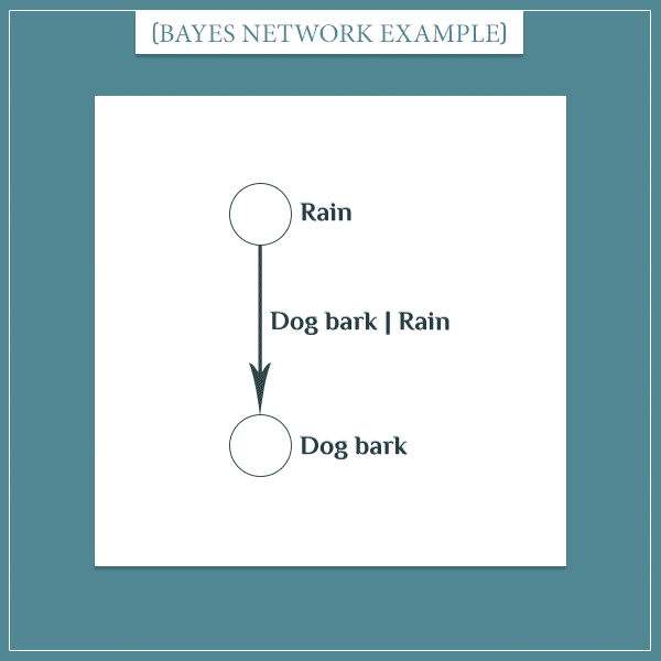
Here’s how the events “it rains/doesn’t rain” and “dog barks/doesn’t bark” can be represented as a simple Bayesian network:
The nodes are the empty circles. Next to each node you see the event whose probability distribution it represents. Next to the arrow is the conditional probability distribution of the second event, given the first event. It reads something like:
- The probability that the dog will start barking, given that it’s currently raining.
In general, the nodes don’t represent a particular event, but all possible alternatives of a hypothesis (or, more generally, states of a variable). In this case, the set of possible events for the first node consists of:
- It rains
- It doesn’t rain
And for the second node:
- The dog barks
- The dog doesn’t bark
But in most cases, the nodes can take more than two and often an infinite number of possible values.
Bayesian networks as joint probability distributions
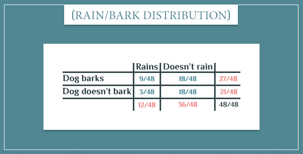
The simple graph above is a Bayesian network that consists of only 2 nodes. It represents a joint probability distribution over their possible values. That’s simply a list of probabilities for all possible event combinations:
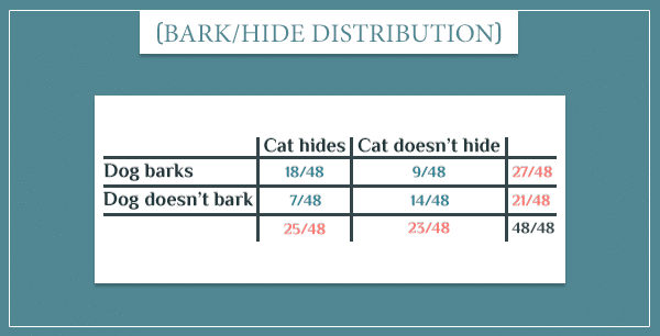
The blue numbers are the joint probabilities of the 4 possible combinations (that is, the probabilities of both events occurring):
Notice how the 4 probabilities sum up to 1, since the four event combinations cover the entire sample space.
The orange numbers are the so-called marginal probabilities. You can think of them as the overall probabilities of the events:
These are obtained by simply summing the probabilities of each row and column. For example, P(Rains) is the probability that it rains, regardless of whether the dog barks or not.
Building complex networks
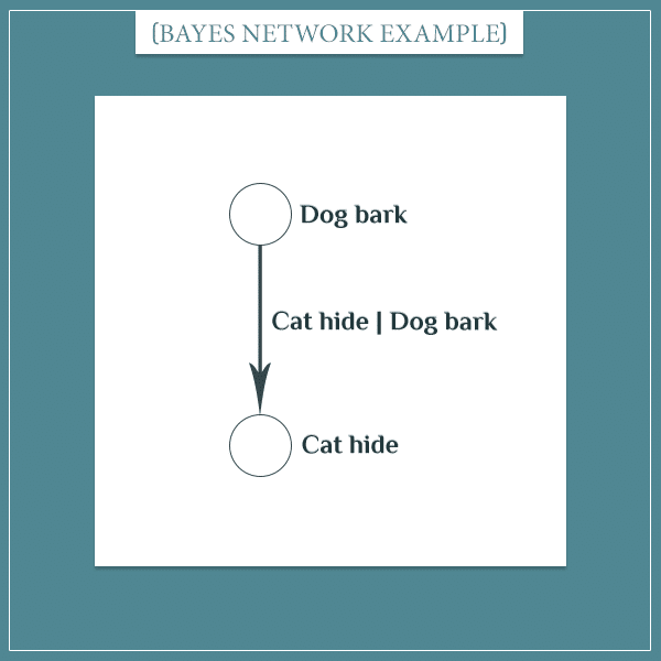
Earlier I mentioned another relationship: if the dog barks, the cat is likely to hide under the couch. Same as before, this relationship can be represented by a Bayesian network:
Here’s the joint probability distribution over these 2 events I came up with:
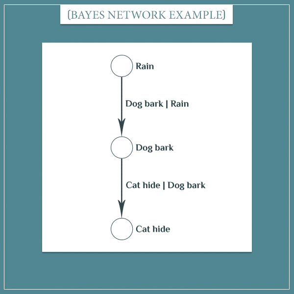
What if you wanted to represent all three events in a single network? Doing this is surprisingly easy and intuitive:
The main idea is that you create a node for each set of complementary and mutually exclusive events (like “it’s raining” and “it’s not raining”) and then place arrows between nodes that directly depend on each other. Each arrow’s direction specifies which of the two events depends on the other.
Networks can be made as complicated as you like:
Each of these nodes has possible states. For example:
- Season: Spring / Summer / Fall / Winter
- Grass: Dry / Wet
- Cat mood: Sleepy / Excited
The arrows hold the probabilistic dependencies between the nodes they connect (I omitted labeling the arrows to not make the graph too cluttered). In other words, for each arrow there’s a table like the ones I showed in the previous section.
For example, the arrow between the “Season” and “Allergies” nodes is a table of joint probabilities. This table will hold information like the probability of having an allergic reaction, given the current season.
What are Bayesian networks used for?
I think it’s most intuitive to think about a Bayesian network as a model of some aspect of the world. The network has certain assumptions about the probabilistic dependencies between the events it models.
You can use Bayesian networks for two general purposes:
- Making future predictions
- Explaining observations
Take a look at the last graph. An example of making a prediction would be:
- If P(Dog bark = True) is high, P(Cat hide = True) is also high.
In other words, if the dog starts barking, this will increase the probability of the cat hiding under the couch.
Explaining observations would be going in the opposite direction. If the cat is hiding under the couch, this will increase the probability that the dog is barking, because the dog’s barking is one of the possible things that can make the cat hide.
Most of the time, you construct Bayesian networks as causal models of reality (although they don’t have to necessarily be causal!). This means that you assume the parents of a node are its causes (the dog’s barking causes the cat to hide).
In the next section, I’m going to show the mechanics of making predictions and explaining observations with Bayesian networks.
Updating probabilities of Bayesian networks
New information about one or more nodes in the network updates the probability distributions over the possible values of each node.
Generally, there are two ways in which information can propagate in a Bayesian network: predictive and retrospective. I’m going to explain both in turn.
Predictive propagation
Predictive propagation is straightforward — you just follow the arrows of the graph. If there’s new information that changes the probability distribution of a node, the node will pass the information to its children. The children will, in turn, pass the information to their children, and so on.
Here’s an example from the last graph. Imagine that the only information you have is that the current season is fall:
(This automatically sets the probabilities of the other possible seasons to 0.)
Here’s an animated illustration of how this information will propagate within the network (click on the image to start the animation):
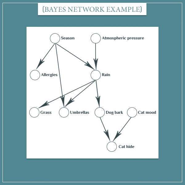
Whenever a node lights up, it means something updated its probability distribution (either external evidence or another node).
Let’s follow one of the information paths. Knowing that the season is fall increases the probability that it’s currently raining. That, in turn, increases the probability that the dog is barking at the window. Finally, that increases the probability that the cat is hiding under the couch.
If this sounds intuitive, it’s because it is. The information propagation simply follows the (causal) arrows, as you would expect.
Retrospective propagation
Retrospective propagation is basically the inverse of predictive propagation. Normally, when something updates a node’s probability distribution, the node also updates its children. But if a node was updated directly or by its child, it also updates its parents.
Here’s an example. Imagine that the only information you have is that the cat is currently hiding under the couch:
Click on the graph below to see another animated illustration of how this information gets propagated:

First, knowing that the cat is under the couch changes the probabilities of the “Cat mood” and “Dog bark” nodes. The intuition is that both can potentially be the cause(s) of the cat hiding. For example, if the cat is hiding under the couch, something must have caused it. This directly makes the probabilities of its potential causes higher.
In the animation, the “Cat hide” node updates its parents one at a time. However, I’m only showing them one at a time because it makes it easier to visually trace the information propagation in the network. In reality, the “Cat hide” node updates the “Cat mood” and “Dog bark” nodes simultaneously. I’m going to explain this in more detail in the second part of this post.
The newly updated “Dog bark” node will now update its own parent, the “Rain” node (again, because the rain is one of the possible reasons for the dog’s barking).
Notice that each updated node also updates its children through predictive propagation. For example, when the “Dog bark” node updates the “Rain” node, the latter updates the “Grass” and “Umbrellas” nodes. That is, now that P(Rain = True) is higher, it’s also more likely that the grass is wet and that people are carrying umbrellas.
It’s also important to note that when you update two or more nodes, they will update their child simultaneously (similar to how a node updates its parents simultaneously).
Summary
Well, this is it for the first part. Here are the main points I covered:
- Bayesian belief networks are a convenient mathematical way of representing probabilistic (and often causal) dependencies between multiple events or random processes.
- A Bayesian network consists of nodes connected with arrows.
- Each node represents a set of mutually exclusive events which cover all possibilities for the node.
- Nodes send probabilistic information to their parents and children according to the rules of probability theory (more specifically, according to Bayes’ theorem).
The two ways in which information can flow within a Bayesian network are:
- Predictive propagation, where information follows the arrows and knowledge about parent nodes changes the probability distributions of their children.
- Retrospective propagation, where information flows in a direction opposite to the direction of the arrows and children update the probability distributions of their parents.
In the second part of this post, I’m specifically going to focus on how this flow of information happens mathematically. And in an informal third part, I’m also going to explain the concept of conditional dependence and independence of a set of nodes, given another set of nodes.
In future posts, I plan to show specific real-world applications of Bayesian networks which will demonstrate their great usefulness.
Stay tuned!
dear SIR,
i have conducted machining process of turning on Inconel material,the parameters we have taken for consideration is Cutting speed,feed rate ,depth of cut ,vibration and after the machininng process we have measured surface roughness offline using stylus instrument,As a part of research we want to work on surface roughness prediction modelling techniques,it seems like Bayes Model is good .We are in initial stage ,i just need your valuable tips and the steps for initiating this work
Hi Abhijith, I’m glad you are finding Bayes networks useful in your research! At what stage of the modeling process are you? I will assume you are still at the planning stage. Have you selected a language/framework you want to write your model in?
Also, please let me know what kind of tips you need most. Are you wondering about the kind of hierarchy your network should have? Also, please provide a bit more details on your data and the kind of relationships different variables have.
Awesome explanation
awesome explanation
Thank you very much. So good.
Hello Cthaeh,
I have been following all your posts on Bayesian networks, and they are excellent and extremely useful. I have quite a few essays to submit over the Easter break, and I want to base almost all of my essays on Bayesian belief networks. I have been trying to think of hypothetical examples and create causal networks for those examples. However, I have not been quite successful in doing so. One of the topics I want to work on is “Information overload and Bayesian networks. We live in complex environments, and the human brain is forced to absorb, observe, and update its prior beliefs based on whatever it sees in the environment. This ability of the brain to update its preferences or beliefs would also depend on the complexity of the information that it acquires. So I want to create a network that illustrates the concepts of information overload and bounded rationality. Another topic that I want to work on is “Bayesian networks to understand people’s social preferences in strategic games. For example, given that I had a prior opinion about person A (I feel that person A is selfish), and given that I was altruistic towards him in the previous trial and that he has reciprocated my kind act in the current trial by giving me back a higher payoff, how would my prior belief about person A’s intentions be updated after I have observed person A’s reciprocity. This example is just to give you an idea about what I have in mind. I am open to any suggestions. I would be thankful to you if you could clue me in on how I can go about the ideas that I have.
Hi Varun, thank you for appreciating my posts, I am very happy that you find them useful!
Can you tell me a bit more about the first topic? For what course are you writing these essays? Do you want the essay to be more philosophical or do you want to include actual (example/hypothetical) calculations?
The second topic sounds very interesting. A straightforward approach to this problem would be something like this. Say you have a population of agents and each agent has some intrinsic strategy. This strategy is going to translate into actual intentions during a specific game, social interaction, etc. For example, let’s say there’s 4 dominant strategies in the population:
– Selfish
– Altruistic
– Tit for tat (TFT)
– Advanced tit for tat (A-TFT)
We can assume some hypothetical prior distribution over these strategies and base it on the frequency of the strategies in the population. For example:
And now let’s say you start interacting (in a game theoretic way) with an unknown opponent, randomly drawn from the population. Say you’re playing a game in which you both take turns to choose between two actions types: “selfish” (S) and “altruistic” (A), with the corresponding payout structure for each combination SS, AA, SA, AS.
Then say you’ve played against your opponent for awhile. Now you have some actual data with your opponent in the form of a particular sequence of actions, represented by pairs (the first in the pair is your action and the second is your opponent’s action). For example, after the first 10 rounds you may have something like this:
R1: AS
R2: AS
R3: AS
R4: SS
R5: SS
R6: SS
R7: AA
R8: AS
R9: AA
R10: AS
In short, let’s call this the data (D):
D = {AS, AS, AS, SS, SS, SS, AA, AS, AA, AS}
And now say you want to calculate the posterior probability of your opponent having the Selfish strategy:
Here P(Selfish) is just the prior probability we specified above. The most difficult part would be to come up with the likelihood term P(D | Selfish). You would need to have a specific model of how you expect Selfish agents (and the remaining 3 strategies) to act. That is, how consistent is the sequence of moves you’ve observed with each strategy?
There are many specific ways to model this and there isn’t any obvious best option, in my opinion. But like I said in the beginning, it depends on the type of essay you would like to write. Is it more on the philosophical or mathematical side? Would you need to build an actual Bayesian network?
Anyway, feel free to ask me any questions regarding what I wrote above!
By the way, not directly related to Bayesian networks, but if you haven’t already, check out this really cool website which allows you to play around and simulate interactions with different social strategies.
Hello Cthaeh,
Thank you very very much for taking your time and giving me such a detailed response. What would be the best way to contact you? I would like to elaborate on what I have in mind.
You can always use the Contact section at the very top of the page.
But I’m sure other readers will find your questions interesting and they can also contribute to the discussion with their own ideas and recommendations. Feel free to write most of what comes to your mind here 🙂
With regard to the first topic, the essay is for a module called ‘|Psychological Models of Choice, which is part of my M.Sc program (I am pursuing an M.Sc in Behavioural and Economic Science).Informational overload has to be the main theme of the essay. I want to make use of some hypothetical calculations. To give you a more clear idea about what I have in mind, standard economic theory presumes that agents are unboundedly rational, and that our brains have the ability to make complex utility computations. However, in reality, the human brain is boundedly rational, and has its own cognitive limitations and boundaries. It is human tendency to have initial beliefs and expectations about what we are going to observe and what we observe in the environment. So given that we live in an ever-demanding world, where a million things happen around us simultaneously, our brain is forced to focus its attention on many things at the same time. It is thus natural for us to miss out on pieces of information that may eventually turn out to be crucial to update our prior beliefs, preferences and expectations about things that we are interested in. What do you think is the best way to illustrate this point? I want to use some kind of causal/bayesian network, but I am not sure as to how to go about it. Can I use Bayesian networks in R and create a model that would demonstrate this combination of informational overload and bounded rationality?
As far as the second topic is concerned, I need to write a 1000-worded essay on ‘Trust and Altruism in games’, which is part of my Experimental Economics module. However, we have not been asked to conduct any experiments and all. We have been instructed to read up a few relevant articles and try to improve on the existing literature. The example that you have given me in your reply post is definitely in concurrence with what I have in mind. As you say, choosing an appropriate model to elucidate our point is the challenging bit. I would be happy if my essay leans more towards the mathematical side. However, I don’t mind looking at it from a philosophical perspective also.
Regarding the first topic, from what you’re describing it sounds like you need a cognitive model that takes into account these cognitive limitations (in attention, working memory, etc.), so a neural network is probably more appropriate than a Bayesian network. I guess one way you can still tie it to Bayes networks is through computational complexity. Here’s some background reading.
Regarding the second topic, you can make several simplifying assumptions in order to create a simple model for illustrative purposes. For example, you can model the probabilities of particular actions, given past actions, as a (n-th order) Markov chain. Check this really good Quora reply to see an example of how you can use Markov chains in Bayesian networks.
Mathematically, these are not trivial concepts and might require a bit time and patience to understand. I am planning to write posts that explain things like Markov models in more digestible manner but for now you would have to mostly rely on other sources.
In the meantime, let me know if you have any specific questions!
Hello Cthaeh,
Are you aware of sources/articles that are based on the application of Markov chain in Bayesian networks apart from the Quora reply that you had asked me to refer to last month?
Hi Varun. Sure! Here’s a few examples of using hidden Markov models for traffic prediction, speech recognition, and hand gesture recognition.
In general, you can search for applications of hidden Markov models (HMM). They don’t necessarily have to be Bayesian, though any non-Bayesian model could be turned Bayesian. Of course, the price you pay is making the model more computationally expensive.
Good explanation! You make it so simple. Thanks a lot ☺
Hello Sir,
I found your post quite helpful. I have a problem in hand where I have some variables describing a disaster world and I need to draw a causal graph using those variables. I need to know how this theorem can help me to do that. From where I can start and build the network using this theorem?
Hi, Diwakar!
I could give the the following rough guidelines. The first step is to build a node for each of your variables. Then whenever there is a causal link between two nodes, draw an arrow from the cause node to the effect node. Your root nodes would be the ones which have no causes within the model. And the leaf nodes would be those that don’t have effects. Usually these are the so-called observation nodes.
In general, following the ideas I presented in this post and the second part should be sufficient for at least constructing the graph. Maybe try to formulate more specific questions, so I know at which steps you may be getting stuck. Also, it would be helpful to give some more background information about the model itself. What the variables are, how they are related to each other, and so on.
This is the clearest explanation I have come across. Many thanks
Hello Cthaeh,
Thank you for a nice blog post. I learned a lot!
I was wondering if you know how to estimate covariance between several “continuous” random variables from a graphical model? Further, calculate the conditional probability between these random variables?
Hi, Rahul! I’m happy you found the post useful!
Regarding your question, when you say several variables, I’m assuming you mean to calculate the covariance between pairs of variables, right? Since covariance is defined between 2 variables only, not several at the same time.
So, how to find the covariance between two continuous random variables taken from a graphical model? I’m going to cover the topic of covariance in a separate post, but for now let me give a quick answer.
Let’s say the two variables (nodes) are labeled A and B. The formula for their covariance is:
Here the operator stands for “expected value“. In other words, the covariance between A and B is equal to the difference: the expected value of
  minus the product of the expected values of A and B. Therefore, to get the covariance, you need to calculate the following three terms and you’re done:
 ![Rendered by QuickLaTeX.com \mathop{\mathbb{E}[A]](data:image/svg+xml,%3Csvg%20xmlns='http://www.w3.org/2000/svg'%20viewBox='0%200%2033%2018'%3E%3C/svg%3E) ,
, ![Rendered by QuickLaTeX.com \mathop{\mathbb{E}[B]](data:image/svg+xml,%3Csvg%20xmlns='http://www.w3.org/2000/svg'%20viewBox='0%200%2034%2018'%3E%3C/svg%3E) , and
, and ![Rendered by QuickLaTeX.com \mathop{\mathbb{E}}[A \cdot B]](data:image/svg+xml,%3Csvg%20xmlns='http://www.w3.org/2000/svg'%20viewBox='0%200%2060%2018'%3E%3C/svg%3E) .
.
Now, if A and B are independent, their covariance is zero (if you haven’t already, check out my post on conditional dependence/independence for Bayesian networks). In other words, if by a graphical analysis you find out that A and B are independent, there’s nothing to calculate.
On the other hand, if the graphical analysis shows that they are dependent, you need to calculate the values of the terms and here’s what each term is equal to:
Here is the joint probability density of A and B. If you’re not sure how to get that from the graph, please take a look at the second part of this post.
Does this make sense? I don’t know your mathematical background and I’m not sure how much detail I should go into. Feel free to ask any further questions.
Hello Cthaeh,
Thank you very much for a detailed explanation. This really helps, I could follow your explanation. Do you know of any python or R package that works with “continuous random variable” for building graphical model? I’m currently building models using pgmpy by discretizing continuous data.
My big aim is to build Bayesian network as shown in this tutorial (PMML_Weld_example : https://github.com/usnistgov/pmml_pymcBN/blob/master/PMML_Weld_example.ipynb)
. Using this tutorial I can estimate the distribution of different random variables. In fact, I can also estimate the “distribution of the covariance” using LKJ prior as shown in this tutorial https://docs.pymc.io/notebooks/LKJ.html. But since pymc3 doesn’t support graphical models, I can’t ask conditional questions to the PMML_Weld_example. Do you know if there is a way?
Can you suggest any handson tutorial or book where continuous variable graphical models are applied to real world data ?
Many thanks!
Yes, I know what you’re looking for Rahul, because I was looking for the same thing in the past 🙂 I don’t think there are Python libraries that do exactly what you want. In fact, some time ago I decided to write one myself, but never got to do that until now. If you are determined enough, you can probably make pymc3 models behave similar to graphical models with some tweaking, but it doesn’t come out of the box.
Regarding your second question, have you read Christopher Bishop’s book Pattern Recognition and Machine Learning? There, chapter 8 is dedicated to graphical models and there’s a lot of problems. The focus isn’t on real-world data per se, but it still presents a wide variety of scenarios.
Otherwise, this website’s destiny is to also include the things you’re currently looking for. I hope I manage to get to completing all the posts I have in mind sooner.
Thank you so much Cthaeh. I’ll read Christopher Bishop’s book.
I happened to come across conditional linear Gaussian graphical models that compute the inverse covariance matrix to generate connections between graphs. I also came across a book Bayesian networks: A practical guide to applications. They have really cool case studies. Unfortunately, the problems are solved using paid software packages. Anyways, I decided to read both these books.
Best wishes for your future blogs.