What Is a Sample Space?

The concept of a sample space is fundamental to probability theory. It is the set of all possibilities (or possible outcomes) of some uncertain process.

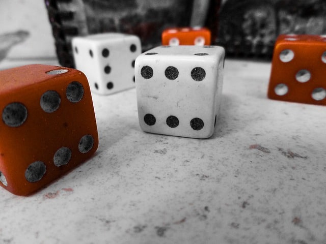
For example, the sample space of the process of flipping a coin is a set with 2 elements. Each represents one of the two possible outcomes: “heads” and “tails”. The sample space of rolling a die is a set with 6 elements and each represents one of the six sides of the die. And so on. Other terms you may come across are event space and possibility space.

Before getting to the details of sample spaces, I first want to properly define the concept of probabilities.

Table of Contents

Probabilities

The probability of an event is a number between 0 and 1 which represents the uncertainty in the event’s occurrence. The notation used for expressing probabilities is P(Event) = X, where X is a number between 0 and 1. For example, when flipping a coin, the probabilities of each outcome are:

$P(\textrm{"Heads"}) = 0.5$

$P(\textrm{"Tails"}) = 0.5$

By the way, if this is the first time you’re seeing this notation, you might want to take a look at my introductory post on Bayes’ theorem, where I also introduce a few basic probability theory concepts. In this section, I am going to define probabilities in a slightly more formal way. For that, I am going to assume you have either read my post or have a basic understanding of events, probabilities, and conditional probabilities.

The axioms

The mathematical definition of probabilities depends on 3 axioms. They are called Kolmogorov’s axioms and are named after the Russian mathematician Andrey Kolmogorov. It was his intuition that all properties of probabilities follow from these simple statements:

P(Event) ≥ 0: The probability of any event is a number greater than or equal to 0.
P(Sample Space) = 1: The probability that at least one of the possible events of a random process will occur is equal to 1. The sample space covers all possible events, and it is certain that at least one event will occur. Therefore, the probability of the entire sample space has to be equal to 1. For example, when flipping a coin, it will either land heads or it will land tails. There is no third possibility, assuming landing on its edge is impossible (or that you re-flip the coin in case that happens).
From a set of non-overlapping events, the probability that at least one event will occur is equal to the sum of the probabilities of the individual events in the set. This one will require the most clarification, even though it’s actually much simpler than it sounds.
Non-overlapping events are events which cannot occur at the same time (like simultaneously flipping both heads and tails). Consider the following example. What is the probability of rolling an even number with a six-sided die? In this case, the outcomes that correspond to the event of rolling an even number are rolling 2, 4, or 6. And notice that they are completely non-overlapping because you cannot roll any pair of numbers simultaneously. Then, according to this axiom, the probability of rolling an even number is:

$P(\textrm{"Even Number"}) = P(\textrm{"Roll 2"}) + P(\textrm{"Roll 4"}) + P(\textrm{"Roll 6"})$

What do these axioms mean?

Earlier, I mentioned the requirement for probabilities to be numbers between 0 and 1. Notice that this is actually a consequence of the first two axioms. The third axiom is intuitive, because you would expect to get 1 after adding the probabilities of all non-overlapping events in the sample space, since they cover the entire set of possible outcomes.

Of course, the full list of consequences of these axioms is quite long and includes all theorems in probability theory (one of the big names in the list is, of course, Bayes’ theorem).

In case you’re wondering how to interpret the fact that these statements are axioms, think about it this way. In order for a set of measures to be probabilities (in the mathematical sense), they need to comply with these three statements. So, the role of the axioms is to basically mathematically distinguish probabilities from non-probabilities.

For a more detailed discussion on the meaning of probabilities, check out this post.

Sample spaces

Imagine a creature which has one special power: given any set of options, it can select one of them in a perfectly unbiased and unpredictable manner.

For example, if you give the creature 5 boxes and ask it to open one of them, the creature will make its choice with no inclination towards any of the boxes. In fact, its decisions are so unpredictable that even the creature itself never knows what they will be before they are actually made. I’ll call this creature Random (you never saw this coming, did you?).

What’s special about Random is that I can use him to build a metaphor for representing processes with probabilistic outcomes. Imagine that Random’s entire existence consists of choosing points on a square whose area is equal to 1:

Notice that I’m not specifying any particular units for the area of the square because, for our purposes, they don’t matter. All that matters is that the area is equal to 1 (well, every square’s area is equal to 1 in some units).

So, Random’s job is choosing points on this square. That’s it. But remember, every time he picks a point, his pick is completely… random. He has no memory of his previous choices. Also, no point on the square has any privilege over the others.

But what does this metaphor have to do with probabilities?

As you’ve probably guessed, this square represents the entire sample space of a random process. Remember, the sample space is the set of all possible outcomes of the process. The square’s area represents the total probability and, therefore, it has to be equal to 1.

A few examples

Imagine that the square is divided into separate regions. Each region represents some set of outcomes of the random process. For example, any process with two equally probable outcomes can be represented by dividing the square in two parts with equal areas.

An example of such a process is flipping a fair coin:

Let’s continue with the metaphor. When you flip the coin, Random’s choice of a point on the square determines the outcome. If the selected point happens to be in the upper half of the square, the coin lands heads; otherwise it lands tails. Notice two things about the areas representing the events “Heads” and “Tails”:

They are equal to each other
Their sum is equal to the area of the square

Since the square represents the entire sample space, the two rectangles associated with the possible outcomes of the coin flip represent their respective probabilities. Therefore, the probability of an event is the fraction of the area of the square which represents the event.

In this case, the areas representing “Heads” and “Tails” are each half of the area of the square. So, the probability for each outcome is the area of the square divided by two: P(“Heads”) = P(“Tails”) = 1/2 (equivalent to 0.5).

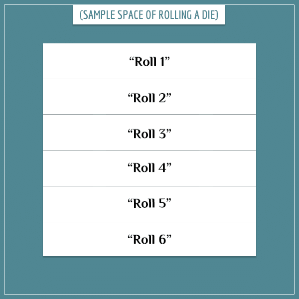
Consider two other examples. The first one is the sample space of rolling a fair die:

Again, the square is divided into equal parts which represent the probabilities of the 6 possible outcomes. Each outcome’s probability is then equal to 1/6.

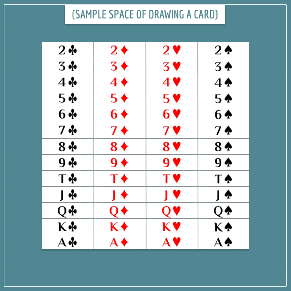
The second example is the sample space of randomly drawing a card from a 52-card standard deck:

This time the square consists of 52 equal parts, each representing a different card from the deck. Therefore, the probability of drawing any one card is 1/52.

To get a better intuition about this assignment of probabilities, check out my introductory post on probability distributions.

Okay, if you managed to follow things so far, you already have a good feeling of sample spaces. One final topic I want to cover in this section is conditional probabilities and how they relate to sample spaces.

Sample spaces and conditional probabilities

The conditional probability of one event, given a second event, is the probability that the first event will occur under the assumption that the second event has already occurred. The most common notation for conditional probabilities is:

$P(\textrm{Event-1} \mathbin{\vert} \textrm{Event-2})$

Imagine that during a particular season of the year, the probability of having a day with a cloudy morning is 0.6 and the probability of a day with a sunny morning is 0.4. Also imagine that the probabilities for the day being rainy or dry are each 0.5:

$P(\textrm{"Cloudy Morning"}) = 0.6$

$P(\textrm{"Sunny Morning"}) = 0.4$

$P(\textrm{"Rainy Day"}) = 0.5$

$P(\textrm{"Dry Day"}) = 0.5$

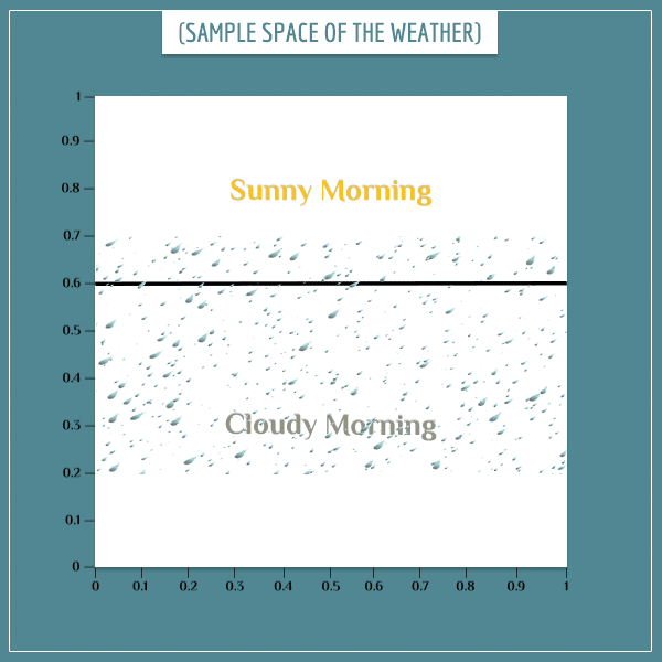
So far I haven’t said anything about the distribution of rainy/dry days among days with cloudy/sunny mornings. In other words, I haven’t specified any of the conditional probabilities, like P(“Rainy Day” | “Cloudy Morning”). I will pick a particular distribution by graphically illustrating the joint sample space of the two events:

Joint sample spaces

Joint sample spaces represent probabilities of combinations of outcomes of two or more uncertain processes. In the current example, there are two such processes: type of day (rainy/dry) and the type of morning (cloudy/sunny). The 4 possible combinations are:

Cloudy morning, rainy day
Cloudy morning, dry day
Sunny morning, rainy day
Sunny morning, dry day

What I essentially did in the image above was to superimpose the sample space of the type of day onto the sample space of the type of morning. The thick black line divides the events of cloudy vs. sunny morning.

For example, the area of “Cloudy Morning” is 6/10 of the area of the entire sample space, so P(“Cloudy Morning”) = 0.6. The white space in the square represents the probability for a dry day.

As you have guessed, the parts of the square marked with rain drops represent rainy days. Don’t worry about the fact that the area for dry day is split. All that matters is the total area that each event covers. In this case, both “Rainy Day” and “Dry Day” cover exactly one half of the area of the square.

Calculating conditional probabilities

Using the sample space, you can now calculate any conditional probabilities you like. Remember that conditional probabilities express the probability of the first event, given the second event. This means that if you know one of the events has occurred, you simply ignore the remaining parts of sample space.

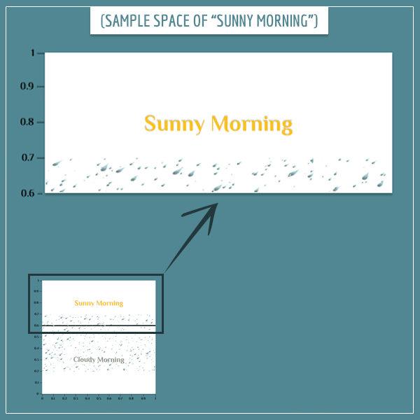
Suppose you see that the morning is sunny and want to calculate the probability that the day will be rainy. Well, here is the sample space for P(“Rainy Day” | “Sunny Morning”):

Because you know the morning is sunny, the part of the old sample space that corresponds to the “Sunny Morning” event becomes the new sample space. And you reevaluate the probabilities of the remaining events according to this new information. Also, because it’s a sample space, its probability has to be equal to 1. Then, notice that the rainy day part now only covers 1/4 of the area of this new sample space (and not 1/2, like in the old sample space):

$P(\textrm{"Rainy Day"} \mathbin{\vert} \textrm{"Sunny Morning"}) = \frac{1}{4} = 0.25$

In the same, way you can calculate the probability of rain when the morning is cloudy:

$P(\textrm{"Rainy Day"} \mathbin{\vert} \textrm{"Cloudy Morning"}) = \frac{4}{6} \approx 0.67$

As an exercise, you can try calculating the remaining conditional probabilities using the same graphical method.

Summary

The sample space (possibility space) is the set of all possible outcomes of some uncertain process. All possible non-overlapping events are like the tiles that cover the sample space. Also, one event may cover more than a single outcome (like the event of rolling an even number with a 6-sided die, which consists of the individual outcomes of rolling 2, 4, or 6).

If you’re new to the topic, I hope you found this post easy to follow. Understanding sample spaces gives you a toolkit for getting your head around more complicated concepts in probability theory, both formally and on an intuitive level.

I use a lot of the ideas and intuition in this post in another post where I show the derivation of Bayes’ theorem. Be sure to check it out!