Mean and Variance of Discrete Uniform Distributions

In today’s (relatively) short post, I want to show you the formal proofs for the mean and variance of discrete uniform distributions. I already talked about this distribution in my introductory post for the series on discrete probability distributions. Well, this is a pretty simple type of distribution that doesn’t really need its own post, so I decided to make a post that specifically focuses on these proofs. More than anything, this is going to be a small exercise in algebra.

This post is part of my series on discrete probability distributions.

In short, you use the discrete uniform distribution when you have n possible outcomes that are equally likely to occur. That is, when the sample space you’re interested in consists of exactly n elements, each of which occupy an equal share of the whole space. Before we look at the mean and variance formulas and their proofs, let’s review (and somewhat generalize) the discrete uniform distribution’s probability mass function (PMF).

Table of Contents

Discrete uniform distribution and its PMF

So, for a uniform distribution with parameter n, we write the probability mass function as follows:

The probability mass function of a discrete uniform distribution with input variable x and parameter n

Here x is one of the natural numbers in the range 0 to n – 1, the argument you pass to the PMF. And n is the parameter whose value specifies the exact distribution (from the uniform distributions family) we’re dealing with. Specifically, the number of possible outcomes. You remember the semi-colon notation for separating parameters (and what parameters are), right? If not, it might be a good idea to review the intro post.

For example, when n = 8, we can plot the probabilities of $\frac{1}{n} = \frac{1}{8} = 0.125$ of the numbers 0 through 7:

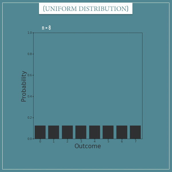
A plot of a discrete uniform distribution with parameter: n = 8

Notice that this distribution doesn’t simply model outcomes which happen to be equally likely. The numbers have to be consecutive! If they aren’t, it would be more appropriate to model the process with a categorical distribution.

In the intro post, I showed you the uniform distribution’s canonical version where the first number is always 0. But, as long as we keep the numbers consecutive, we can shift the distribution to the left or to the right. For example, here’s the same distribution shifted 4 numbers to the right:

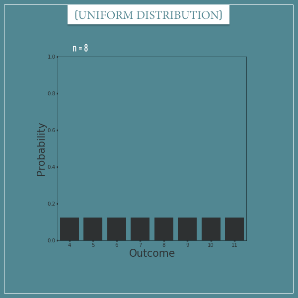
A plot of a shifted discrete uniform distribution with parameter: n = 8

If we’re dealing with a shifted distribution, we need to specify an additional parameter for the starting value. Today I want to use the letter L (for “lower bound“) for this parameter:

The probability mass function of a discrete uniform distribution with input variable x and parameters L and n

Notice that the canonical version is a special case of this more general version with L = 0.

Yet a third way to parameterize this distribution is by also specifying the upper bound parameter U:

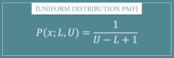
The probability mass function of a discrete uniform distribution with input variable x and parameters L and U

Notice that specifying L and U automatically determines n because:

$n = U - L + 1$

In the example above, $L = 4$

, $U = 11$

, and $n = 11 - 4 + 1 = 8$

For another example, consider the distribution with parameters $L = 1$ and $U = 36$ with which you can model the probability of the pocket the ball will land in for a particular roulette spin.

Mean and variance formulas

So, here I’m going to give you the standard formulas for the mean and variance of a uniform distribution with parameters n or L and U. I’m going to use $\mu$ (the Greek letter mu) for the mean and $\sigma^2$ (the Greek letter sigma squared) for the variance.

Those are the most common notations for these two measures. In particular, $\sigma^2$ is based on $\sigma$ , which is how standard deviation is typically denoted. You remember the relationship between variance and standard deviation from my introductory post on measures of dispersion, right?

Anyway, here are the two formulas for the canonical version of the distribution:

$\mu = \frac{n-1}{2}$

$\sigma^2 = \frac{n^2 - 1}{12}$

The variance formula for the more general (shifted) version is the same as the one above. On the other hand, the mean formula has a small modification:

$\mu = \frac{n-1}{2} + L$

That is, we simply add the lower bound parameter L to the canonical mean, again with the understanding that $n = U - L + 1$

Proofs of mean and variance formulas

Before I show you the proofs, I’m want to list a few properties and identities we’re going to need to understand them. The first two concern the mean and variance of an arbitrary shifted distribution:

$\mu(X + c) = \mu(X) + c$

$\sigma^2(X + c) = \sigma^2(X)$

What these identities say is that shifting an arbitrary random variable by adding an arbitrary constant c to all of its possible values has the following effect on the mean and variance:

The mean gets shifted by c
The variance remains the same

Since I haven’t talked about these properties before, I’m going to show you their proofs in the bonus section at the end of this post. For now, just take my word for it. These two properties will allow us to easily generalize the mean and variance formulas from the canonical version of a uniform distribution to its general (arbitrarily shifted) form.

And here’s the remaining properties and identities we’re going to need.

Auxiliary properties and identities

First, you should feel comfortable with properties of arithmetic operations. In particular the familiar commutative and associative properties of addition and multiplication, as well as the distributive property of multiplication over addition. All these properties state that, for arbitrary numbers a, b, and c:

$a + b = b + a$

$a \cdot b = b \cdot a$

$a + (b + c) = (a + b) + c$

$a \cdot (b \cdot c) = (a \cdot b) \cdot c$

$a \cdot (b + c) = a\cdot b + a \cdot c$

Second, we’re going to rely on the following two properties of the sum operator (derived from the arithmetic properties above):

(1) $\begin{equation*} \sum_{i} c \cdot x_i = c \cdot \sum_{i} x_i \end{equation*}$

(2) $\begin{equation*} \sum_{i} (x_i + y_i) = \sum_{i} x_i + \sum_{i} y_i \end{equation*}$

Third, we’re going to need the following closed-form formulas (which I also talked about in the sum operator post):

(3) $\begin{equation*} \sum_{i=0}^{n} i = \frac{n(n+1)}{2} \end{equation*}$

(4) $\begin{equation*} \sum_{i=0}^{n} i^2 = \frac{n(n+1)(2n+1)}{6}\] \end{equation*}$

Finally, we’re going to need the following alternative variance formula of a random variable X:

(5) $\begin{equation*} \sigma^2(X)} = \mathop{\mathbb{E}[X^2] - \mathbb{E}[X]^2 \end{equation*}$

Where $\mathbb{E}[.]$

is the expected value notation.

If all these properties (and notation) are new to you, I recommend you review the posts I linked to so far, where you’ll find everything explained in detail.

And with all that out of the way, let’s finally get to the proofs we’re interested in!

The mean

To calculate the mean of a discrete uniform distribution, we just need to plug its PMF into the general expected value notation:

$\sum_{i=0}^{n-1} x_i \cdot P(x_i) = \sum_{i=0}^{n-1} i \cdot \frac{1}{n}$

Then, we can take the $\frac{1}{n}$

factor outside of the sum using equation (1):

$\sum_{i=0}^{n-1} i \cdot \frac{1}{n} = \frac{1}{n} \cdot \sum_{i=0}^{n-1} i$

Finally, we can replace the sum with its closed-form version using equation (3):

$\frac{1}{n} \cdot \sum_{i=0}^{n-1} i = \frac{1}{n} \cdot \frac{n(n-1)}{2}$

$= \frac{n-1}{2}$

And there you have it, we just derived the mean formula I showed you in the previous section!

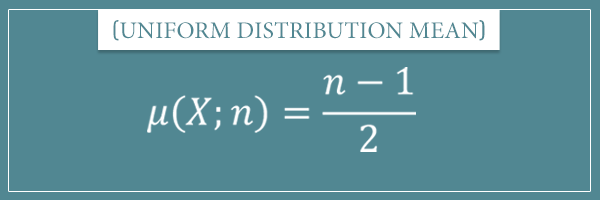
The mean formula for a uniform distribution with input variable x and parameter n

Notice that we slightly modified the closed-form expression for the sum with the following substitutions:

$n \Rightarrow n-1$
$n+1 \Rightarrow n$

That is because in our case the sum runs from 0 to n – 1, instead of from 0 to n (as in equation (3)).

Were you expecting a more complicated proof? Well, maybe not.

So, this is the mean formula for the canonical version whose lower bound L is 0. Using the mean of a shifted distribution identity I gave above, we can generalize the mean for any lower bound L:

$\mu(X) = \frac{n-1}{2} + L$

To get more intuition about this formula, let’s add the two terms and replace n with $U - L + 1$

$\mu(X) = \frac{n-1}{2} + \frac{2L}{2}$

$= \frac{n-1 + 2L}{2}$

$= \frac{(U - L + 1) - 1 + 2L}{2}$

$= \frac{L + U}{2}$

You’ll commonly see this version of the formula, which shows that the mean of the distribution is nothing but the arithmetic mean of the lower and upper bounds!

The variance

Now let’s do the derivation for the variance of a discrete uniform distribution formula. We’re going to use the alternative variance formula from equation (5):

$\sigma^2(X)} = \mathop{\mathbb{E}[X^2] - \mathbb{E}[X]^2$

Let’s start with the second term because it’s easier. This is simply the square of the mean we just derived:

$\mathbb{E}[X]^2 = \left(\frac{n-1}{2}\right)^2$

$= \frac{(n-1)^2}{4}$

$= \frac{n^2 - 2n + 1}{4}$

Now let’s focus on the second term by first taking the $\frac{1}{n}$

out using equation (1):

$\mathop{\mathbb{E}[X^2] = \sum_{i=0}^{n-1} i^2 \frac{1}{n}$

$= \frac{1}{n} \sum_{i=0}^{n-1} i^2$

Then, we can substitute the sum with the right-hand side of equation (4) and simplify:

$\frac{1}{n} \sum_{i=0}^{n-1} i^2= \frac{1}{n} \frac{n(n-1)(2n-1)}{6}$

$= \frac{(n-1)(2n-1)}{6}$

$= \frac{2n^2 - 3n + 1}{6}$

So, now that we have simple expressions for the two terms, we can plug them into equation (5) and do the final simplification:

$\sigma^2(X) = \mathop{\mathbb{E}[X^2] - \mathbb{E}[X]^2$

$= \frac{2n^2 - 3n + 1}{6} - \frac{n^2 - 2n + 1}{4}$

$= \frac{4n^2 - 6n + 2}{12} - \frac{3n^2 - 6n + 3}{12}$

$= \frac{4n^2 - 6n + 2 - 3n^2 + 6n - 3}{12}$

$= \frac{n^2 - 1}{12}$

And we reached the expected result!

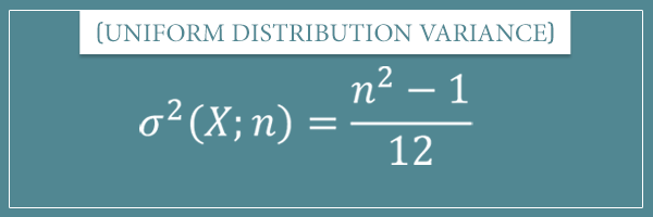
The variance formula for a discrete uniform distribution with input variable x and parameter n

See how easy these proofs are when we already have the proper tools at hand?

And since shifting a random variable doesn’t change its variance, this is also the formula for the general discrete uniform distribution.

You could also express the formula in terms of L and U:

$\sigma^2(X) = \frac{(U - L + 1)^2 - 1}{12}$

$= \frac{L^2 + U^2 + 2(U - L - LU)}{12}$

Though the representation in terms of n is definitely more elegant (and preferable)!

Summary

Well, this is it for today. The discrete uniform distribution is one of the simplest distributions and so are the proofs of its mean and variance formulas.

The special and general probability mass functions of this distribution look like this:

$P(x; n) = \frac{1}{n}$

$P(x; L, U) = \frac{1}{U - L + 1}$

And the mean and variance formulas whose derivation I showed you are:

$\mu(X) = \frac{n-1}{2}$

$\sigma^2(X) = \frac{n^2 - 1}{12}$

The general variance formula looks exactly the same, whereas the general mean formula takes a small modification:

$\mu(X) = \frac{n-1}{2} + L = \frac{L + U}{2}$

Anyway, if you had any issues with following the derivations, don’t hesitate to ask your questions in the comment section below!

Now, as I promised, for the curious among you I’m going to show the proofs for the mean and variance identities regarding shifted random variables.

Bonus section

As you saw, the proofs for the mean and variance of discrete distributions are very short and easy to follow. Well, this is also because we had other (previously proved) identities at our disposal.

On the other hand, the direct proofs of the general version of the distribution are a bit hairy. For that reason, in this bonus section I want to show you the proofs of two general facts about the mean and variance of an arbitrary shifted discrete distribution. These were the facts that allowed us to immediately adapt the special case proofs to the general case (and circumvent the hairy direct proofs).

Basically, to shift a distribution simply means adding an arbitrary constant c to every value of the sample space. In the example in the beginning, we shifted the canonical uniform distribution (with parameter n = 8) 4 numbers to the right by adding the constant c = 4 to every value in the range 0 to 7 (and the new range became 4 to 11).

Now let’s see what happens to the mean and variance of any discrete distribution, not just the one we’re currently looking at.

Mean of a shifted random variable

As a reminder, here’s the general formula for the expected value (mean) a random variable X with an arbitrary distribution:

$\mathbb{E}[X] = \mu(X) = \sum_{i} x_i p(x_i)$

Notice that I omitted the lower and upper bounds of the sum because they don’t matter for what I’m about to show you. Assume that the sum ranges over all values in the sample space.

Now let’s create a new random variable Y which is the shifted version of X by an arbitrary constant c:

$Y = X + c$

And let’s write an expression for its mean:

$\mathbb{E}[Y] = \mathbb{E}[X + c] = \mu(X + c) = \sum_{i} (x_i + c) p(x_i)$

Now, using the commutative and distributive properties of multiplication, as well as identities (1) and (2) from above, we can rewrite the right-hand side as follows:

$\sum_{i} (x_i + c) p(x_i) = \sum_{i} \left(x_i p(x_i) + c p(x_i)\right)$

$= \sum_{i} x_i p(x_i) + \sum_{i} c p(x_i)$

$= \mu(X) + c\sum_{i} p(x_i)$

$= \mu(X) + c$

In the third line, we replaced $\sum_{i} x_i p(x_i)$

with $\mu(X)$

and in the fourth line we replaced $\sum_{i} p(x_i)$

with 1 because the sum of all elements in the sample space is always equal to 1. Therefore, the mean of a random variable shifted by c is simply the mean of the unshifted version itself shifted by c:

$\mu(X + c) = \mu(X) + c$

Cool. Now let’s see how things work with the variance.

Variance of a shifted random variable

As a reminder, here’s the canonical variance formula:

$\sigma^2(X) = \sum_{i} (x_i - \mu(X))^2 p(x_i)$

Now, let’s apply it on the shifted version of X:

$\sigma^2(X + c) = \sum_{i} \left[(x_i + c) - \mu(X+c)\right]^2 p(x_i)$

$= \sum_{i} \left[(x_i + c) - (\mu(X) + c)\right]^2 p(x_i)$

$=\sum_{i} (x_i + c - \mu(X) - c)^2 p(x_i)$

$= \sum_{i} (x_i - \mu(X))^2 p(x_i) = \sigma^2(X)$

In the second line I simply replaced $\mu(X+c)$

with $\mu(X) + c$

(which we just derived). And in the third line I simply expanded the inner parentheses. The net result is that the constant c got cancelled out and we’re left with the original expression. Which means that shifting a random variable doesn’t change its variance!