Predicting the 2016 US Presidential Election

November 7 UPDATE: click here to view our final update post where we give our latest analyses just a day before the election!
Click here to go to our daily predictions page.

In the first 10 posts I mostly concentrated on theoretical topics. But the general focus of this blog is much broader. For the first time I’m going to show an actual application of probability theory for estimating real life events.

An ongoing event many people are closely following right now is the US presidential election. The primary season officially concluded at the end of July and now the general election battle is in full swing. The main clash is between former Secretary of State Hillary Clinton (D) and businessman Donald Trump (R). Clinton and Trump are challenged by 3^rd party candidates Gary Johnson from the Libertarian Party (a two-time former governor of New Mexico) and Jill Stein from the Green Party (a physician and a political activist).

Introduction

I worked with my friend and classmate Luca on a model that predicts the evolution of voter preferences in time. More specifically, the model uses presidential election polls to estimate what voter preferences for all 4 candidates would be on election day (the 8^th of November). We estimate voter preferences in all states and use them to calculate the probability of each candidate winning each state. Finally, we use the state win probabilities to calculate each candidate’s probability of winning the entire presidential election and becoming the next US president.

Luca is currently doing a PhD in cognitive neuroscience. He has serious interest in machine learning and time series analysis and is currently developing new algorithms in neuroscience and other fields. You can check out his personal page in Google Scholar.

The model we worked on is an example of an application of a machine learning method.

You can see the current model predictions in the very first section below. They are followed by an overview of how US presidential elections work in general. In the main part of this post, I’ll go over the details of our model and the way we use it to make these predictions. Finally, I’m going to conclude the post with some general thoughts on the current election cycle.

Our 2016 predictions

Without further ado, take a look at the latest predictions of our model. To view results for other dates, click on the date above the map. The explanations are below the map.

The color of each state on the map shows the candidate who is a favorite to win it. The candidate colors are:

• Red: Donald Trump
• Blue: Hillary Clinton
• Green: Jill Stein
• Yellow: Gary Johnson

The intensity of each state’s color represents how certain the favorite is to win. That is, states with paler colors are less predictable than those with solid colors.

The three tables below the map show:

• The electoral votes each candidate is currently expected to win.
• The probability of each candidate winning the majority of the electoral votes (270 or more).
• The probability of each candidate winning the highest number of electoral votes without necessarily reaching 270.

In case no candidate reaches the 270 electoral vote threshold, the US Congress will determine the winner of the presidential election. You can find a detailed explanation of the general election process in the next section.

You can see our current estimates for candidate preferences by clicking on the tabs below the map. The plots show the candidate preferences’ evolution in time. The colored circles in the single-candidate plots show all the polls the estimates are based on. The poll sample size is color-coded according to the legend on the right.

You can click on individual states to see the state-specific predictions of our model.

Finally, you can see our model’s predictions from previous dates by clicking on the date above the map.

How the presidential election process works

In a little over a month and a half, eligible US voters will choose the next US president. However, unlike many Western democracies, the US president is not directly elected by voters. Instead, the president is chosen by an institution called the United States Electoral College.  This institution currently consists of 538 electors who choose the president about a month after the November vote. Each elector casts a single vote and the presidential candidate who gets 270 or more votes (i.e., a 50%+ majority) wins the election.

There are three questions that need clarification:

1. Who are these electors and why are they exactly 538?
2. How do they vote?
3. What happens if no candidate gets 270 or more electoral votes?

Here are the answers.

The US Electoral College

The Electoral College consists of 538 electors. This number comes from the number of members of the US Congress. There are currently 535: 435 in the House of Representatives and 100 in the Senate. The additional 3 electors are given to the District of Columbia, which is not a state and has no representation in Congress.

The Electoral College is completely independent of Congress but the number of electors given to a state is strictly equal to that state’s number of legislators. The number is proportional to the population of the state and, consequently, large states like California and Texas have a much bigger influence on the election than small states like Delaware and Montana.

Here’s how electors are distributed across all states:

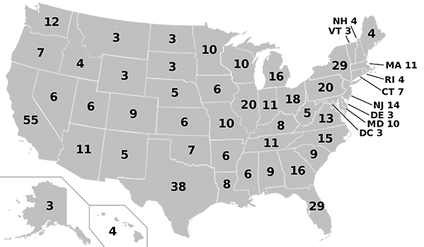
How the Electoral College votes

The 538 electors never actually meet. Electors from each state vote locally a month after election day and their votes eventually reach Congress to be processed along the electoral votes from other states.

Electors from a state cannot split their votes. That is, all electors (with the exception of Maine and Nebraska) vote for the same candidate. Namely, for the candidate who wins the popular vote of the state.  This is essentially a winner-takes-all system where a candidate only needs a plurality win to secure all electors of a state. Maine and Nebraska are somewhat of an exception, since the winner-takes-all system there is applied on a congressional district level, not on a state level (so each of their 4 electors can, in principle, vote for a different candidate).

Technically, there is no text in the US Constitution that forces electors to follow their state’s rules and vote for the winner candidate. An elector’s vote against the popular vote will still be legitimate. However, in practice this almost never happens and some states even have local laws against so-called faithless electors.

Congress breaks the tie

A candidate needs to get at least half of the electoral votes to win the presidential election. In case no candidate passes the 270-elector threshold , the US Congress chooses the next US president and vice president. More specifically, the House of Representatives chooses the president and the Senate chooses the vice president.

The eligible candidates the House can vote for are the top 3 candidates who won the highest number of electoral votes. There’s also the requirement that a candidate needs to win at least one state to be considered in the Congress vote. As for the vice presidential vote, the options before the Senate are limited to the top 2 vice presidential candidates.

If it comes to that, Congress will continue to vote until a candidate receives a majority of the votes. It’s important to note that the 435 representatives don’t vote separately. Instead, all representatives of each state get a single vote. So, California’s 53 representatives will have the same impact on the result of the vote as, say, Alaska’s single representative. To become president, a candidate needs at least 26 of the 50 available House votes.

Alright, enough small talk. Let’s go to the actual predictions for the 2016 election.

The math behind our presidential election predictions

Predicting the presidential election outcome means calculating the probability of each candidate winning the presidency. You can think of a candidate’s win as an event. If you haven’t already, check my introductory post on Bayes’ theorem where I explain the concepts of events and probabilities of events. In the current context, we represent the events of winning the presidency with the following notation:

• P(“Hillary Clinton becomes the next US president”) = 0.7

This says that Hillary Clinton has a 70% probability of winning the election. However, I will use a more compact notation and write the probabilities simply as:

• P(Clinton)
• P(Johnson)
• P(Stein)
• P(Trump)

In order to calculate these probabilities, let’s reduce them to a series of smaller events. We can say:

• P(Clinton) = P(“Clinton wins at least 270 electoral votes”)

Now, to be really strict, the actual probability is:

• P(Clinton) = P(“Clinton wins at least 270 electoral votes OR Clinton finishes in top 3 and Congress votes her in”)

However, in our analysis we don’t model the preferences of Congress and assume that the probabilities of legislators choosing a particular candidate are more or less proportional to the number of electoral votes the candidate won. In other words, the assumption is that not including Congress in our model doesn’t have a significant effect on our predictions. Given the very small chance of no candidate getting 270+ electoral votes in this election, this is most likely not going to be relevant at all.

Okay, let’s delve deeper into the analysis.

Probability of 270+ electoral votes

There are many ways for a candidate to win 270+ electoral votes. The probability of this event is equal to the probability that the candidate wins a combination of states whose sum of electors is greater than or equal to 270. An example of such a combination is:

1. New Jersey (14)
2. North Carolina (15)
3. Georgia (16)
4. Michigan (16)
5. Ohio (18)
6. Illinois (20)
7. Pennsylvania (20)
8. Florida (29)
9. New York (29)
10. Texas (38)
11. California (55)

A candidate who wins these 11 states will have exactly 270 electoral votes and win the presidential election.

Okay, we’re making progress. So far, a candidate’s probability of becoming president looks like this:

• P(Candidate) = P(“Candidate wins a combination of states whose sum of electors ≥ 270”)

The next logical step is to calculate the candidate probabilities of winning each of the 51 states (yes, the District of Columbia technically isn’t a state). After that, each candidate’s general election probability can be calculated by following these steps:

1. Calculate the probabilities of all state combinations.
2. Take all combinations with 270+ electors and calculate the portion of the sample space they occupy.

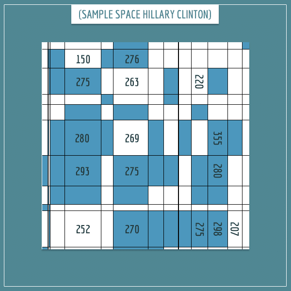
The electoral college sample space

If you’re hearing the term ‘sample space’ for the first time, check out my post about sample spaces. In short, a sample space is the set of all possibilities of a random experiment or a random process. In our case, the elements of the sample space are the possible state combinations. The random process is the voting on election day itself. For each candidate, the probability of winning more than 270 electors is simply the portion of the sample space occupied by the “270+” combinations.

The figure above shows an example representation of Hillary Clinton’s sample space. Each rectangle stands for one combination of states. Its area represents the probability of her winning that particular combination. Rectangles colored in blue are combinations that pass the threshold of 270 electors. The size of each rectangle is proportional to the probability of Clinton winning that combination. Her overall probability of winning the election is equal to the sum of the areas of blue rectangles divided by the total area of the sample space.

Remember, each rectangle represents a combination like “Nevada, New Jersey, Oklahoma…”. The numbers associated with rectangles are the sums of electors a candidate would get if they won exactly that combination.

Notice that the areas of rectangles don’t depend on the number of electors in the combinations. The sample space consists of all possible combinations and two separate combinations which result in the same number of electoral votes may have very different probabilities for a candidate. Combinations mainly consisting of deep red states like Mississippi and Louisiana will be very unlikely for Clinton but very likely for Trump to win.

How we calculate candidate win probabilities

The figure above is an extremely simplified representation of a candidate’s real sample space. You can see that it only has about 150 rectangles. However, the actual number of possible state combinations is huge and impossible to represent visually. In case you’re curious, the exact number is:

•  2⁵¹ = 2 251 799 813 685 248

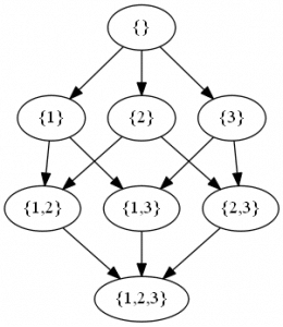
This is the number of all subsets of the 51 states, also known as the power set (you can see how the number is reached in my post on combinatorics).

So, we’re interested in the probability of the compound event of winning one of the 270+ state combinations. This probability equals the sum of the probabilities of these special combinations. However, given the huge number of possibilities, calculating each combination’s probability would literally take forever. So, we took a simpler approach.

We decided to approximate the probability by simulating the presidential election multiple times. We calculated each candidate’s win probability as the number of times they crossed the 270 threshold, divided by the total number of simulations. These kinds of approximations are common in fields like machine learning and statistics, when calculating the exact probability is infeasible because it involves summing a very large number of terms.

One simulation is basically having virtual voters express their preferences. In each simulation, each candidate wins or loses a state with the probability we calculated with our model. Then, we sum the electors from all the states the candidate won. If the number passes the 270 threshold, the candidate’s win count increases by 1. A candidate’s win probability is their win count divided by the total number of simulations we run.

A description of our model

Estimating state win probabilities

This is the main and most important part of our model.

We use two sources of information in estimating the state-level candidate probabilities:

1. The state and national poll results (which we take from the website RealClearPolitics)
2. The demographic characteristics of states

The polls inform us about the voter preferences for candidates. What we need to do is use these preferences to calculate the probability of each candidate winning each state.

So, how do we do that?

A common mistake is to equate a candidate’s win probability with their respective preference. In other words, if 53% of the polled likely voters in a state said they preferred Trump, this doesn’t mean Trump will win the state with a probability of 0.53. In fact, if we knew with absolute certainty that 53% of the voters would vote for Trump, his win probability would be 1 and everybody else’s would be 0.

From presidential election polls to probabilities

Can’t we just take the average of all polls for a particular state? And declare the candidate with the largest preference the most likely winner?

There are two problems with this approach. First, the polls are inherently noisy because they are taken over samples and not over the entire population. Their results can never be taken at face value. Second, and more importantly, the preferences for each candidate evolve over time. Some voters change their preferences from one candidate to another or change their mind about voting versus not voting in the first place.

The number of votes a candidate receives is inherently a random and uncertain quantity. We need to somehow estimate the likely distribution of preferences on election day based on the available polls at any point in time. This is what such an estimation looks like:

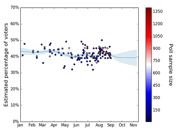
This is an example plot which shows our estimation for Hillary Clinton’s national preferences in the first days of September. The approach for estimating state preferences is identical.  The circles show the poll results and their colors indicate the poll sample size. The thick line shows the expected (mean) percentage of voters for Clinton. The shaded area around the line represents the range of most probable values (the variance) according to our predictor — the ones closer to the line being more probable than the ones further away.

Estimating future voter preferences

We model the evolution of the preferences as Gaussian processes. The details of this part of the analysis are quite advanced, however. For now, what you need to know is that our model is capable of detecting trends in the poll results and uses them to estimate candidate preferences in future time points.

We use the state demographic data to transfer information between states. We use the following information (per state) to calculate a similarity matrix between all states:

• Age and sex
• Educational attainment
• Median household income
• Party and political affiliation
• Race and ethnicity
• Religion
• Sexual orientation
• Unemployment rate
• Results from the previous election

This similarity matrix allows information to “flow” between states. A state poll will update the estimates not only for the state in which it was taken, but also for states with similar demographics. To give an example, a poll in Alabama will have a larger effect on the estimates of another red state like Kansas than on a blue state like Massachusetts. I’m going to leave the exact details of this for a future post.

We calculate the state win probabilities using a similar method to the one we used for simulating the entire election. Namely, we draw samples from the estimated distribution of preferences on election day, count the number of times a candidate had the highest preference, and divide by the total number of draws.

In the final section of this part of the post, I am going to demonstrate the reliability of our model by showing its accuracy in “predicting” the 2012 presidential election outcome.

Validation of the model on the 2012 presidential election

Below is the map showing the results of the 2012 election followed by our model’s predictions based on all 2012 state and national polls.

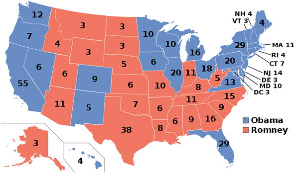
By clicking on any of the months below, you can see what our predictions would have been on that particular month.

February | March | April | May | June | July | August | September | October | November | Latest

Our model shows that Obama was a huge favorite to win the election throughout the entire cycle, despite him being neck-to-neck with Romney according to the national polls. This is a perfect illustration of how the Electoral College renders winning the national popular vote almost useless.

Notice that we correctly predict the favorite to win every state, except for Florida (even though some of our early predictions do correctly give Florida to Obama). A possible explanation for this discrepancy could have something to do with pollster biases we didn’t take into account. Or this could simply be a surprising result too. Small probability events do occur (in fact, they occur all the time).

The overall accuracy of our predictions gives us great confidence in our estimates of this year’s election.

General thoughts on the 2016 presidential election

Hillary Clinton and Donald Trump are the favorites to win the presidency. However, there are 2 other serious players in this election: Gary Johnson and Jill Stein. Although their chances of winning are currently very low, they are the only other candidates who have a theoretical chance of winning the election. By ‘theoretical chance’ I mean that they are going to be on the ballot in enough states to be able to win at least 270 electoral votes.

Also, even if they don’t win, they can have a significant effect on the election outcome if they manage to “steal” enough votes from Trump or Clinton. Especially if they do so disproportionately and in key states.

The unusual election

Many people, including myself, think that this year’s US presidential election is among the most interesting elections in recent US history.

The main reason is that there have been significant shifts in the political preferences among US voters in a relatively short amount of time. Maybe it’s more accurate to say that the election cycle so far has revealed shifts in the political spectrum many people were unaware of. These were shown by both the Democratic and Republican primary elections, as well as the general election campaigns.

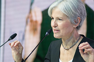
For starters, nobody expected 3^rd party candidates’ current popularity. In the 2012 election, Gary Johnson received about 1% of the national vote. Now, just 4 years later, he is polling at around 10%! Similarly, Jill Stein received less than 0.5% of the vote in 2012 but now she is polling at around 4-5%.

This can be partly explained by the fact that the two main candidates have a strongly polarizing effect on voters. Both Hillary Clinton and Donald Trump have very high unfavorability ratings and many voters vow to never vote for one or either of them. Naturally, this led to the rise of popularity of other candidates, as many voters started looking for alternatives.

Attitudinal changes among voters have deeper roots than disaffection with the two main candidates alone. A Gallup analysis published earlier this year showed a record high number of voters identifying as political independents. So, it’s more accurate to say that the disaffection is actually with the two-party system that has been dominant in US politics for the past 2 centuries, as well as with the two major parties themselves.

The unexpected candidates

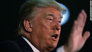
It first became clear that this election was going to be different from previous ones by the surprisingly big popularity of candidates who people perceived as “anti-establishment”.

On the Republican side, Donald Trump started out with small poll numbers but quickly established himself as the front-runner in the primaries — a position he held all the way to the Republican National Convention in July.

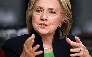
On the Democratic side, Hillary Clinton started the race as a big favorite but ended up having to fight for her nomination against Bernie Sanders, who was the “anti-establishment” candidate in the Democratic primaries. Sanders surprised voters and pundits by closing a 50% gap in the polls and gave Clinton a very hard time throughout the primary season. Unlike Trump, Sanders didn’t get the Democratic nomination, but his popularity is likely to have a significant effect on the election outcome. Despite being out of the race, he is still campaigning for Clinton and against Trump. He also managed to shift some of Clinton’s positions on important issues like healthcare, education, and campaign financing.

The number of eligible US voters is around 250 million, of which about 50% are likely voters. The voter turnout in this election is expected to be higher than usual, due to the factors I discussed above. I expect the election to get even more intriguing and unpredictable in its final stages, especially when the candidates go head-to-head in the debates.

Summary

Here’s a recap of the 4 main steps to arriving at our final election forecast:

1. Estimate the likely range of voter preferences for each candidate on election day using polls and state demographics.
2. Calculate each candidate’s probability of winning each state
3. Using these probabilities, simulate the election a large number of times.
4. Calculate each candidate’s probability of winning the election as the percentage of simulations in which the candidate won 270 or more electoral votes.

The accuracy of these predictions depends on the assumption that the polls are relatively unbiased towards candidates. Also, note that at any point in time there may be an event or multiple events which drastically shift the trends of the election. Such events may be a big political blunder, a leaked revelation, or another type of political scandal which involves one or more candidates. Keeping in mind how this election has unfolded so far, such events aren’t all that unlikely. Especially if we remain to see the best of this election for last!

Our model does quite well in “predicting” the 2012 election results, so we are optimistic about the accuracy of its predictions for the current presidential election too. We are looking forward to comparing the election results to our predictions at different points in time.

All in all, we have an exciting month and a half ahead of us!

---

Special thanks to Sparx, Veli, and Meryl for their contribution to the writing of this post!